24/5/24 - initial long-form draft for review & discussion
28/6/24 - first released version 30/4/25 - updated with data up to & including half term 4 of the 2024/25 school year
1 Introduction
This document is an assessment of Special Educational Needs (SEN) in Sheffield children. There follows an analysis of volumes of pupils with different levels of need and different specific needs; how this is changing over time; comparisons with other authorities; the demographic makeup of children with SEN; geographical distributions and differences in prevalence; links to economic deprivation; school attendance, attainment and exclusion; and the types of support offered within the city.
The data used comes from the Sheffield School Census; Capita One attendance and exclusion records; and published government data.
Important
This report remains in draft, and the figures here are subject to revision & change
2 Summary of key points
Around 1 in 5 pupils in Sheffield has some level of SEN, and almost 1 in 20 have an EHC plan in place
This figure is growing over time, with a particular increase seen since the COVID-19 pandemic
Among core cities, Sheffield has around the average level of children with an EHC plan, but above average prevalence of children with SEN support
The most prevalent specific needs are also the fastest growing, these are:
Speech, language & communication needs (SLCN)
Social, emotional & mental health needs (SEMH)
Autism
Moderate learning difficulty
Children who have an EHC plan are more likely to be male, and peak in Y7
The majority of children with SLCN are boys in the early primary years, and as these children age the cohort is likely to grow significantly
There is increased prevalence among certain ethnic groups
There is a strong apparent link to economic deprivation
Children with SEN have lower rates of school attendance, particularly in secondary phase
Children with SEN support experience a bigger drop off in attendance between years 6 and 7
All SEN levels see a steeper decline during secondary school that children without SEN
Attendance rates are worsening over time for children with SEN support
3 Overall volumes
Special Educational Needs pupils in Sheffield - Spring 2025
data from School Census & Capita One attendance records; counts rounded to nearest 10
all pupils
primary
secondary
count
%
count
%
count
%
No SEN
61500
81.4%
31330
81.2%
24640
79.4%
SEN Support
10880
14.4%
5870
15.2%
4650
15.0%
EHCP
3160
4.2%
1380
3.6%
1730
5.6%
As of the half term period ending 2025-03-28 there were 13649 pupils between years 1 and 11 with SEN support or an EHC plan in place. This is 19.6% of all pupils. Of these, 89% are in mainstream provision.
3.1 Growth over time
The numbers of pupils with SEN support and with EHC plans have been growing year on year, with a significant rise in the years following the COVID pandemic.
Caution
At the time of writing levels of both categories seem to have reduced on the previous year. This may reflect data availability, or delays to assessments rather than true prevalence
4 Types of school provision
4.1 Mainstream and special
Of primary age pupils with an EHC Plan, around 30% are placed in special schools. In secondary this figure is 48.5%.
Pupils with an EHC plan in Sheffield, by provision type
count of pupils on roll in Spring 2025; data from School Census & Capita One attendance records
mainstream
special
count
%
count
%
Primary
893
66.7%
446
33.3%
Secondary
771
48.3%
825
51.7%
4.2 Elective Home Education (EHE) and Education Other than at Setting (EOTAS)
Elective Home Education & Education Other Than Setting Data
The EHE & EOTAS data is from a separate source to the pupil counts for mainstream & special above. There is potentially some overlap & figures here are provisional
Pupils educated other than in mainstream or special
count of pupils registered as EOTAS or EHE on 1/4/2024; data from Capita One & school census
Education other than setting
Elective Home Education
EHCP
Primary
3
16
Secondary
21
29
SEN Support
Primary
-
51
Secondary
-
104
The numbers of electively home educated children continue to grow dramatically - though noteably not for those with an EHC plan.
Volumes of children with an EHC plan who are educated other than at setting also continue to rise dramatically:
4.3 Alternative Provision
Pupils with special educational needs in alternative provision
count of pupils registered to Sheffield Inclusion Centre on 1/4/2025; data from Capita One & school census
Sheffield Inclusion Centre
SEN Support
Primary
6
Secondary
126
EHCP
Primary
6
Secondary
29
5 Benchmarking
Taking published DfE data to compare Sheffield to the other core cities, and Sheffield’s statistical neighbours.
Caution
Since we are looking at published DfE data here, the figures here may not align with other areas of this report that use local data.
Sheffield has slightly more EHCP and SEN support pupils than the core cities average.
Sheffield also has slightly more children with an EHC plan than our statistical neighbours.
For SEN support, Sheffield is higher than all our statistical neighbours.
6 Primary Specific Needs
The most common specific needs are Speech, Language and Communication needs, Social Emotional and Mental health, and Autism.
Note
This chart looks significantly different to the previous year, see the time series chart below to see the changes in more detail.
A primary specific need is recorded in the school census data for pupils with SEN support or an EHCP. Here we look at volumes over time, and for clarity, we have divided these into two plots. The first shows the larger groups (pupil count >= 1000). There has been substantial growth in the prevalence of three specific needs: Speech, Language and Communication Needs; Social, Emotional & Mental Health; and Autism.
Heading into 2025, SLCN has continued to grow dramatically, while the autism and SEMH categories have reduced.
This second plot shows the smaller groups (pupil count < 1000), these smaller groups are mostly static in prevalence, except a noteable reducting in severe learning difficulties Note that 2020 has been removed from these plots due to COVID shutdowns affecting the data.
7 Age & gender
Age & gender profiles show a significant gender bias towards males in the SEN cohorts. There is a particular peak in EHCP rates for boys in Y7. SEN support volumes are higher in Primary Provision.
8 Ethnicity
8.1 Time series of ethnicity
This time series displays the count of children requiring SEN support or an EHC plan for broad ethnic groups, and shows some differences in rates of growth and decline.
Pupils in Sheffield, by ethnicity description and SEN level
count of pupils on roll in 2024/25; data from School Census & Capita One attendance records
EHCP
SEN Support
No SEN
Total
count
% of row
count
% of row
count
% of row
all pupils
3414
4.7%
11500
15.7%
58267
79.6%
73181
White British
2062
5.0%
7120
17.3%
32056
77.7%
41238
Black African and White/Black African
267
4.3%
653
10.5%
5308
85.2%
6228
Pakistani
232
4.2%
773
14.0%
4518
81.8%
5523
Any Other Ethnic Group
118
3.8%
401
12.7%
2627
83.5%
3146
Any Other White Background
105
3.8%
344
12.4%
2315
83.8%
2764
White/Black Caribbean
136
6.9%
437
22.2%
1399
70.9%
1972
Other Asian Background
77
4.1%
202
10.8%
1586
85.0%
1865
Gypsy, Roma and Traveller of Irish Heritage
56
3.3%
527
31.1%
1113
65.6%
1696
White/Asian
77
4.6%
221
13.2%
1381
82.3%
1679
Any Other Mixed
63
3.9%
268
16.5%
1298
79.7%
1629
not known
81
5.6%
166
11.5%
1196
82.9%
1443
Indian
26
2.0%
61
4.8%
1191
93.2%
1278
Bangladeshi
30
3.6%
113
13.6%
687
82.8%
830
Any Other Black Background
37
4.8%
90
11.6%
646
83.6%
773
Chinese
18
2.8%
39
6.0%
590
91.2%
647
Black Caribbean
24
6.5%
71
19.3%
272
74.1%
367
Irish
5
4.9%
14
13.6%
84
81.6%
103
9 Mapping
The following maps show the prevalence, per 100 or 1000 pupils of the following SEND characteristics: EHCP; SEN support; Speech, language & Communication needs; Social, Emotional & Mental Health needs; Autism; physical disabilities; learning difficulties; visual impairment; hearing impairment and multi-sensory impairment.
The maps show how these prevalence rates vary across the wards of the city. Note that this is based on ward of residence rather than school attended. Rates have been calculated for pupils on roll during the 2024/25 academic year and for all pupils in years 1 to 11. In a change to previous versions of this report, the maps on specific needs now include those with secondary specific needs as well as primary needs - though the impact of this change is small.
Education, Health & Care Plans
Sen Support
Speech, Language & Communication Needs
Social, Emotional & Mental Health Needs
Autism
Physical disabilities
Learning Difficulties
Note
The map below shows the prevalence of all learning difficulties listed in the school census data: moderate, specific, severe, and profound & multiple.
Visual Impairment
Hearing impairment
Multi-sensory impairment
10 Deprivation
Measures of deprivation correlate strongly with the prevalence of special educational needs, more so for SEN support, and less so for pupils with an EHCP.
Caution
The apparent prevalences seen here probably result from differences in the true prevalences of SEN in the population, but may also reflect differences in engagement with the system, recording or policy. It is difficult to quantify the relative contributions of these factors from the data, though discussion of these issues with teachers, SEN workers and others on the front line may provide insight.
Some wards seem to have lower SEN levels than might be expected from their deprivation measures alone, and appear below the main groupings on these charts - most noteably Darnall, Burngreave and Firth Park. Other wards appear to have higher prevalence than expected from deprivation measures alone, appearing above the main groupings: e.g. Birley, Beighton, Park & Arbourthorne.
Note that due to it’s low population, city ward is often an outlier on plots such as these.
The relationship between deprivation and speech, language & communication needs is particularly strong.
…and less pronounced for social, emotional & mental health needs, with some signficant outliers, particularly Darnall.
For autism, any link to deprivation is weak:
11 Attendance
On average, school attendance is lower for children with SEN Support, and lower still for pupils with an EHC plan. These differences are greater in secondary schools than in primary, and the drop in attendance levels for SEN support children in secondary is particularly concerning.
Plotting attendance over time by sen level shows how the attendance gap between primary and secondary age children widened after the pandemic. We can also see the gap widen between children with & without SEN. By 2024 an attendance gap of almost 10% had opened up between secondary age children with no SEN and those on SEN support; children with an EHCP plan were attending almost 12% lower. The post pandemic period saw a drop in attendance for all children, but the group with the biggest reduction was children in secondary schools who require SEN Support.
Important
At the time of writing, the last year has seen encouraging recovery in attendance for all groups shown here. The biggest improvements for those groups most heavily affected - secondary school pupils on SEN support or with EHCP plans.
Plotting attendance by national curriculum year and SEN level produces three profiles of attendance. Here we see that the transition to secondary school has the most severe impact on attendance for children requiring SEN support. And while all children see a decline in average attendance through secondary, the decline is more severe for children requiring SEN support. Pupils with an EHC plan show a steady decline from NCY 3 onwards, and no discernable step down into secondary.
12 Attainment
Attainment data is available by SEN level and local authority from the DfE. Here we look at how attainment at Key Stage 2 (KS2) and Key Stage 4 (KS4) differs by SEN status, how Sheffield compares with the core cities, and how this is changing over time. There are many different measures of attainment in the published data, but here we focus on two: - At KS2, the % of pupils meeting expected standard in reading, writing and maths. - At KS4, the average attainment 8 score, which measures attainment across a pupil’s eight best subjects.
At both KS2 and KS4, children with SEN support have lower attainment than those no SEN, and children with EHC plans have lower attainment still.
Comparing with core cities, Sheffield shows similar performance at KS2 to the average for SEN support and children with no SEN, but benchmarks poorly for children with an EHC plan. It’s worth noting that there is large variation in the EHC plan attainment data here, that looks too great to be the result of local policy alone.
At KS4, Sheffield benchmarks around the average for children with an EHC plan, but poorly for those with SEN support.
For the years heavily affected by COVID, the DfE have not published the KS2 expected standard measure we used above, but the available data shows changes over time. Between 2019 and 2022 all children see a drop in attainment at KS2, and all see an improvement into 2023, but both SEN support and EHC plan children show a lesser drop to 2022 and a better recovery into 2023 than children with no SEN.
Finally on attainment, and at KS4 attainment peaking in 2021 and dropping slowly for all SEN groups.
13 Exclusions
Exclusion rates remain very low in primary schools, but rates are consistently higher for SEN support pupils. There has also been a recent rise in fixed period exclusions for primary aged children with an EHC plan.
Exclusion rates in Secondary are rising dramatically both for pupils with no SEN, and those with SEN support (where, just as in primary, rates have always been higher), though not for those with an EHC plan.
The above charts show the rates per 10,000 pupils, so for completion here we include a table of the underlying numbers for 2023/24:
Exclusion rates in Sheffield by SEN level and school phase
counts of exclusions and pupils on roll in 2023/24; data from School Census & Capita One attendance records
primary
secondary
exclusions
pupils on roll
exclusions per 10,000 pupils
exclusions
pupils on roll
exclusions per 10,000 pupils
No SEN
Fixed Period
535
32464
164.8
8474
25878
3274.6
Permanent
11
32464
3.4
111
25878
42.9
SEN Support
Fixed Period
471
6588
714.9
2549
4692
5432.7
Permanent
6
6588
9.1
33
4692
70.3
EHCP
Fixed Period
58
1359
426.8
56
1634
342.7
Permanent
2
1359
14.7
-
-
-
14 Distance to school
Children with SEN may travel further to access a special school, or a more suitable school. We calculated the straight line distance between home and school postcodes, in order to create the following distance profiles. Primary age children live closer to their school than secondary age children, with Over 40% of secondary age children with an EHC plan live over 5km from school.
Source Code
---title: "Sheffield SEND Strategic Needs Assessment"author: "Giles Robinson"version: 0.2date: 2024-08-19editor: visualformat: html: code-tools: true code-fold: true toc: true toc-location: left toc-depth: 3 number-sections: true fig-cap-location: top other-links: - text: Back to SCC Data Science site home href: https://scc-data-science.sheffield.gov.uk/execute: warning: false message: false echo: falseknitr: opts_chunk: out.width: "100%"---### Release notes {.unlisted}24/5/24 - initial long-form draft for review & discussion\28/6/24 - first released version 30/4/25 - updated with data up to & including half term 4 of the 2024/25 school year```{r}#| label: setup#| include: false# clear the environmentremove(list =ls())# load packageslibrary(tidyverse)library(janitor)library(lubridate)library(ggtext)library(ggrepel)library(gghighlight)library(kableExtra)library(MetBrewer)library(corrplot) library(ggcorrplot)#library(shadowtext)library(readxl)library(ggstatsplot)library(geosphere)library(ggridges)library(forecast)library(tsibble)library(scales)library(gt)library(lemon)library(tidytext)# specify data folderdata_folder <-str_c("S:/Public Health/Policy Performance Communications/Business Intelligence/Projects/EIP/data/inclusion/")# copy to excel functioncopy_excel <-function(input) {write.table(input, file ="clipboard-20000", sep ="\t", row.names = F)}# ggplot themeseb <-element_blank()# Set default ggplot themetheme_set(theme_classic() +theme(#plot.title = element_text(),plot.subtitle =element_text(size =10, face ="italic"),plot.caption =element_text(size =8, face ="italic"),plot.title.position ="plot",plot.title =element_markdown(size =12) ))# theme for minimal bar chartsbarplottheme_minimal <-theme(axis.title.y = eb,axis.line.y = eb,axis.ticks.y = eb,axis.line.x = eb,axis.ticks.x = eb)# theme for minimal facetsfacet_theme_minimal <-theme(strip.background = eb,axis.line = eb,axis.ticks = eb,legend.position ="bottom",legend.title = eb,axis.title.x = eb,axis.text.x =element_text(size =7))# Connect to OSCAR database via ODBCoscar_con <- DBI::dbConnect( odbc::odbc(),Driver ="Oracle in OraClient12Home1",Dbq ="SCPRFLVE",UID =if (Sys.getenv("oscar_userid") =="") { rstudioapi::askForPassword("OSCAR User ID") } else {Sys.getenv("oscar_userid") },PWD =if (Sys.getenv("oscar_pwd") =="") { rstudioapi::askForPassword("OSCAR Password") } else {Sys.getenv("oscar_pwd") },timeout =10)# Connect to LCS database via ODBClcs_con <- DBI::dbConnect( odbc::odbc(),Driver ="SQL Server Native Client 11.0",Server ="shef-biprd-01.syhapp.com, 1438", Database ="HDM_Local",UID =if (Sys.getenv("lcs_userid") =="") { rstudioapi::askForPassword("LCS User ID") } else {Sys.getenv("lcs_userid") },PWD =if (Sys.getenv("lcs_pwd") =="") { rstudioapi::askForPassword("LCS Password") } else {Sys.getenv("lcs_pwd") },timeout =10)# # ## connect to LAS database via ODBC# las_con <- DBI::dbConnect(# odbc::odbc(),# #dsn = "LAS",# Driver = "SQL Server Native Client 11.0",# Server = "shef-biprd-01.syhapp.com, 1436",# Database = "HDM",# UID = if (Sys.getenv("las_userid") == "") {# rstudioapi::askForPassword("LAS User ID")# } else {# Sys.getenv("las_userid")# },# PWD = if (Sys.getenv("las_pwd") == "") {# rstudioapi::askForPassword("LAS Password")# } else {# Sys.getenv("las_pwd")# },# timeout = 10# )# summarising attendance function# this is copied from the attendance & exclusion data model.# any changes made there should be reflected here & vice versa# note that the groupings appear TWICE in this function, once for grouped data and once for the "no grouping" scenario (grouping_vars = "none"). Any changes must be consistent across both.summarise_attendance <-function(input_data, grouping_vars) {ifelse (grouping_vars =="none", {# Aggregate without grouping result <- input_data |>mutate(zero_attendance =if_else(present ==0, 1, 0)) |>summarise(child_count =n_distinct(stud_id, na.rm =TRUE),row_count =n(),possible_sessions =sum(possible_sessions, na.rm =TRUE),present =sum(present, na.rm =TRUE),authorised =sum(authorised, na.rm =TRUE),unauthorised =sum(unauthorised, na.rm =TRUE),missing =sum(missing, na.rm =TRUE),excluded =sum(excluded, na.rm =TRUE),family_holiday_agreed =sum(family_holiday_agreed, na.rm =TRUE),family_holiday_not_agreed =sum(family_holiday_not_agreed, na.rm =TRUE),family_holiday_total =sum(family_holiday_total, na.rm =TRUE),illness =sum(illness, na.rm =TRUE),med_appt =sum(med_appt, na.rm =TRUE),no_reason =sum(no_reason, na.rm =TRUE),late_absent =sum(late_absent, na.rm =TRUE),late_pres =sum(late_pres, na.rm =TRUE),late_total =sum(late_absent, na.rm =TRUE) +sum(late_pres, na.rm =TRUE),study_leave =sum(study_leave, na.rm =TRUE),approved_offsite =sum(approved_offsite, na.rm =TRUE),fixed_exclusions =sum(fixed_exclusions, na.rm =TRUE),perm_exclusions =sum(perm_exclusions, na.rm =TRUE),total_exclusions =sum(total_exclusions, na.rm =TRUE),persistent_absent_count =sum(persistent_absence, na.rm =TRUE),severe_absent_count =sum(severe_absence, na.rm =TRUE),zero_attendance_count =sum(zero_attendance, na.rm =TRUE) ) |>mutate(percent_present = present / possible_sessions,percent_auth_absence = authorised / possible_sessions,percent_unauth_absence = unauthorised / possible_sessions,percent_missing = missing / possible_sessions,percent_family_holiday_agreed = family_holiday_agreed / possible_sessions,percent_family_holiday_not_agreed = family_holiday_not_agreed / possible_sessions,percent_family_holiday = family_holiday_total / possible_sessions,percent_excluded = excluded / possible_sessions,percent_illness = illness / possible_sessions,percent_med_appt = med_appt / possible_sessions,percent_no_reason = no_reason / possible_sessions,percent_late_absent = late_absent / possible_sessions,percent_late_pres = late_pres / possible_sessions,percent_late_total = late_total / possible_sessions,percent_study_leave = study_leave / possible_sessions,percent_approved_offsite = approved_offsite / possible_sessions,pc_of_pupils_persistent_absent = persistent_absent_count / row_count,pc_of_pupils_severely_absent = severe_absent_count / row_count,pc_of_pupils_zero_attendance = zero_attendance_count / row_count ) |>mutate(percent_absent =1- percent_present) }, {# Group by specified variables and then summarize result <- input_data |>mutate(zero_attendance =if_else(present ==0, 1, 0)) |>group_by(across(all_of(grouping_vars))) |>summarise(child_count =n_distinct(stud_id, na.rm =TRUE),row_count =n(),possible_sessions =sum(possible_sessions, na.rm =TRUE),present =sum(present, na.rm =TRUE),authorised =sum(authorised, na.rm =TRUE),unauthorised =sum(unauthorised, na.rm =TRUE),missing =sum(missing, na.rm =TRUE),excluded =sum(excluded, na.rm =TRUE),family_holiday_agreed =sum(family_holiday_agreed, na.rm =TRUE),family_holiday_not_agreed =sum(family_holiday_not_agreed, na.rm =TRUE),family_holiday_total =sum(family_holiday_total, na.rm =TRUE),illness =sum(illness, na.rm =TRUE),med_appt =sum(med_appt, na.rm =TRUE),no_reason =sum(no_reason, na.rm =TRUE),late_absent =sum(late_absent, na.rm =TRUE),late_pres =sum(late_pres, na.rm =TRUE),late_total =sum(late_absent, na.rm =TRUE) +sum(late_pres, na.rm =TRUE),study_leave =sum(study_leave, na.rm =TRUE),approved_offsite =sum(approved_offsite, na.rm =TRUE),fixed_exclusions =sum(fixed_exclusions, na.rm =TRUE),perm_exclusions =sum(perm_exclusions, na.rm =TRUE),total_exclusions =sum(total_exclusions, na.rm =TRUE),persistent_absent_count =sum(persistent_absence, na.rm =TRUE),severe_absent_count =sum(severe_absence, na.rm =TRUE),zero_attendance_count =sum(zero_attendance, na.rm =TRUE) ) |>mutate(percent_of_pupils = child_count /sum(child_count, na.rm =TRUE),percent_present = present / possible_sessions,percent_auth_absence = authorised / possible_sessions,percent_unauth_absence = unauthorised / possible_sessions,percent_missing = missing / possible_sessions,percent_family_holiday_agreed = family_holiday_agreed / possible_sessions,percent_family_holiday_not_agreed = family_holiday_not_agreed / possible_sessions,percent_family_holiday = family_holiday_total / possible_sessions,percent_excluded = excluded / possible_sessions,percent_illness = illness / possible_sessions,percent_med_appt = med_appt / possible_sessions,percent_no_reason = no_reason / possible_sessions,percent_late_absent = late_absent / possible_sessions,percent_late_pres = late_pres / possible_sessions,percent_late_total = late_total / possible_sessions,percent_study_leave = study_leave / possible_sessions,percent_approved_offsite = approved_offsite / possible_sessions,pc_of_pupils_persistent_absent = persistent_absent_count / row_count,pc_of_pupils_severely_absent = severe_absent_count / row_count,pc_of_pupils_zero_attendance = zero_attendance_count / row_count )|>mutate(percent_absent =1- percent_present) } )return(result)}percent_calc <-function(input_data){input_data |>tally() |>mutate(freq = n /sum(n)) |>mutate(l_ci = freq - (1.96*sqrt((freq * (1- freq)) / n)),u_ci = freq + (1.96*sqrt((freq * (1- freq)) / n)) )}presence_mean_calc <-function(input_data){input_data |>summarise(mean.percent_present =mean(percent_present, na.rm =TRUE),sd.percent_present =sd(percent_present, na.rm =TRUE),n.percent_present =n() ) |>mutate(se.percent_present = sd.percent_present /sqrt(n.percent_present),lower.ci.percent_present = mean.percent_present -qt(1- (0.05/2), n.percent_present -1) * se.percent_present,upper.ci.percent_present = mean.percent_present +qt(1- (0.05/2), n.percent_present -1) * se.percent_present)}summarise_avg <-function(input_data){ summarise (input_data, mean.percent_present =mean(percent_present, na.rm =TRUE),sd.percent_present =sd(percent_present, na.rm =TRUE),n.percent_present =n() ) |>mutate(se.percent_present = sd.percent_present /sqrt(n.percent_present),lower.ci.percent_present = mean.percent_present -qt(1- (0.05/2), n.percent_present -1) * se.percent_present,upper.ci.percent_present = mean.percent_present +qt(1- (0.05/2), n.percent_present -1) * se.percent_present ) }percent_calc <-function(input_data){input_data |>tally() |>mutate(freq = n /sum(n)) |>mutate(l_ci = freq - (1.96*sqrt((freq * (1- freq)) / n)),u_ci = freq + (1.96*sqrt((freq * (1- freq)) / n)) )}presence_mean_calc <-function(input_data){input_data |>summarise(mean.percent_present =mean(percent_present, na.rm =TRUE),sd.percent_present =sd(percent_present, na.rm =TRUE),n.percent_present =n() ) |>mutate(se.percent_present = sd.percent_present /sqrt(n.percent_present),lower.ci.percent_present = mean.percent_present -qt(1- (0.05/2), n.percent_present -1) * se.percent_present,upper.ci.percent_present = mean.percent_present +qt(1- (0.05/2), n.percent_present -1) * se.percent_present)}``````{r load data}#| label: load data#| include: false# load the whole data modelload(str_c(data_folder,"attendance_inclusion_data_model.RData"))```## IntroductionThis document is an assessment of Special Educational Needs (SEN) in Sheffield children. There follows an analysis of volumes of pupils with different levels of need and different specific needs; how this is changing over time; comparisons with other authorities; the demographic makeup of children with SEN; geographical distributions and differences in prevalence; links to economic deprivation; school attendance, attainment and exclusion; and the types of support offered within the city.The data used comes from the Sheffield School Census; Capita One attendance and exclusion records; and published government data.::: callout-importantThis report remains in draft, and the figures here are subject to revision & change:::## Summary of key points- Around 1 in 5 pupils in Sheffield has some level of SEN, and almost 1 in 20 have an EHC plan in place- This figure is growing over time, with a particular increase seen since the COVID-19 pandemic- Among core cities, Sheffield has around the average level of children with an EHC plan, but above average prevalence of children with SEN support- The most prevalent specific needs are also the fastest growing, these are: - Speech, language & communication needs (SLCN) - Social, emotional & mental health needs (SEMH) - Autism - Moderate learning difficulty- Children who have an EHC plan are more likely to be male, and peak in Y7- The majority of children with SLCN are boys in the early primary years, and as these children age the cohort is likely to grow significantly- There is increased prevalence among certain ethnic groups- There is a strong apparent link to economic deprivation- Children with SEN have lower rates of school attendance, particularly in secondary phase- Children with SEN support experience a bigger drop off in attendance between years 6 and 7- All SEN levels see a steeper decline during secondary school that children without SEN- Attendance rates are worsening over time for children with SEN support## Overall volumes```{r}#| label: calculate overall volumes#| fig-width: 1#| fig-height: 1#| message: FALSE#| warning: FALSE# latest ht end date - for displaying in line belowlatest_ht_end_date <- attend |>filter(ht_id ==max(ht_id)) |>select(ht_id) |>distinct() |>left_join(term_calendar_full) |>select(period_end_date) |>pull()sen_overall_count <- attend |>filter(ht_id ==max(ht_id), ncy >=1, ncy <=11, sen_level %in%c("EHCP","SEN Support") ) |>select(stud_id) |>distinct() |>tally() |>pull()overall_pupil_count <- attend |>filter(ht_id ==max(ht_id), ncy >=1, ncy <=11#,#sen_level %in% c("EHCP","SEN Support") ) |>select(stud_id) |>distinct() |>tally() |>pull()sen_percent_of_pupils <- sen_overall_count / overall_pupil_countsen_mainstream_count <- attend |>filter(ht_id ==max(ht_id), ncy >=1, ncy <=11, sen_level %in%c("EHCP","SEN Support"), school_type =="mainstream" ) |>select(stud_id) |>distinct() |>tally() |>pull()sen_mainstream_percent <- sen_mainstream_count / sen_overall_countall <- attend |>filter(ht_id ==max(ht_id)) |>group_by(sen_level) |>summarise(pupil_count =n_distinct(stud_id)) |>mutate(freq =percent(pupil_count /sum(pupil_count), accuracy =0.1),pupil_count =round(pupil_count,-1)) |>rename(#"SEN level" = sen_level,"all_pupils_count"= pupil_count,"all_pupils_percent"= freq) pri <- attend |>filter(ht_id ==max(ht_id), ncy >=1, ncy <=11, phase =='Primary') |>group_by(sen_level) |>summarise(pupil_count =n_distinct(stud_id)) |>mutate(freq =percent(pupil_count /sum(pupil_count), accuracy =0.1),pupil_count =round(pupil_count,-1)) |>select(-sen_level) |>rename('primary_count'= pupil_count,'primary_percent'= freq) sec <- attend |>filter(ht_id ==max(ht_id), ncy >=1, ncy <=11, phase =='Secondary') |>group_by(sen_level) |>summarise(pupil_count =n_distinct(stud_id)) |>mutate(freq =percent(pupil_count /sum(pupil_count), accuracy =0.1),pupil_count =round(pupil_count,-1)) |>select(-sen_level) |>rename('secondary_count'= pupil_count,'secondary_percent'= freq) table_data <-bind_cols(all,pri,sec)table_data |>gt(rowname_col ="sen_level" ) |>tab_spanner(id =1, label ="all pupils", columns = dplyr::contains("all_pupils")) |>tab_spanner(id =2, label ="primary", columns = dplyr::contains("primary")) |>tab_spanner(id =3, label ="secondary", columns = dplyr::contains("secondary")) |>cols_label(contains("count") ~"count",contains("percent") ~"%" ) |>tab_header(title ="Special Educational Needs pupils in Sheffield - Spring 2025",subtitle ="data from School Census & Capita One attendance records; counts rounded to nearest 10" ) |>tab_options(table.align ="left",heading.title.font.size =12,heading.subtitle.font.size=10,heading.align ="left",column_labels.font.size =14,stub.font.size =12 ) |>cols_align("left",'sen_level' )```As of the half term period ending `r latest_ht_end_date` there were `r sen_overall_count` pupils between years 1 and 11 with SEN support or an EHC plan in place. This is `r scales::percent(sen_percent_of_pupils, accuracy = 0.1)` of all pupils. Of these, `r scales::percent(sen_mainstream_percent, accuracy = 1.0)` are in mainstream provision.### Growth over timeThe numbers of pupils with SEN support and with EHC plans have been growing year on year, with a significant rise in the years following the COVID pandemic.::: callout-cautionAt the time of writing levels of both categories seem to have reduced on the previous year. This may reflect data availability, or delays to assessments rather than true prevalence:::```{r}#| label: plot sen_level volumes over time#| warning: FALSE#| message: FALSEplot_data <- attend |>filter(sen_level !="No SEN") |>group_by(year, sen_level) |>summarise(pupil_count =n_distinct(stud_id)) |>mutate(freq =percent(pupil_count /sum(pupil_count), accuracy =0.1)) |>ungroup() |>mutate(label =if_else(year ==max(year), #str_c( sen_level#,"\n", pupil_count) , NA_character_)) #|> ggplot(plot_data,aes( x = year,y = pupil_count,colour = sen_level,label = label)) +geom_point() +geom_line() +geom_label_repel(nudge_y =-50,nudge_x =0.2,size =3,fontface ="bold",min.segment.length =Inf)+geom_text(data = plot_data #|> filter(year %in% c(2016,2020,2025)), aes(label = pupil_count), size =2.6, vjust =-0.6) +scale_x_continuous(limits =c(2016,2025), breaks =seq(2016,2025)) +labs(title ="Special educational needs in Sheffield",subtitle ="count of pupils on roll in each school year by SEN level",caption ="data from Sheffield School Census & Capita One attendance records") +theme(legend.position ="none", axis.title = eb, axis.line = eb, axis.ticks = eb)```## Types of school provision### Mainstream and specialOf primary age pupils with an EHC Plan, around 30% are placed in special schools. In secondary this figure is 48.5%.```{r}#| label: table of EHCP pupil counts in mainstream and special#| message: FALSE#| warning: FALSEvols_phase_prov <- attend |>filter(ht_id ==max(ht_id), ncy >=1, ncy <=11, phase %in%c("Primary","Secondary"), sen_level %in%c("EHCP","SEN Support"),!is.na(school_type), school_type !=0, school_type !="not applicable",!base_id %in%c(377,1000029808) # remove any pupils in EHE or EOTAS; we're counting those separately below ) |>group_by(sen_level, phase, school_type) |>summarise(pupil_count =n_distinct(stud_id)) |>mutate(percent =percent(pupil_count /sum(pupil_count), accuracy =0.1))table_data <- vols_phase_prov |>filter(sen_level =="EHCP") |>ungroup() |>select(-sen_level) |>pivot_wider(names_from ="school_type",values_from =c("pupil_count","percent") ) |>relocate(contains("mainstream"), .after ="phase") #table_data |>gt(rowname_col ="phase" ) |>tab_spanner(id =1, label ="mainstream", columns = dplyr::contains("mainstream")) |>tab_spanner(id =2, label ="special", columns = dplyr::contains("special")) |>#tab_spanner(id = 3, label = "secondary", columns = dplyr::contains("secondary")) |> cols_label(contains("count") ~"count",contains("percent") ~"%" ) |>tab_header(title ="Pupils with an EHC plan in Sheffield, by provision type",subtitle ="count of pupils on roll in Spring 2025; data from School Census & Capita One attendance records" ) |>tab_options(table.align ="left",heading.title.font.size =12,heading.subtitle.font.size=10,heading.align ="left",column_labels.font.size =14,stub.font.size =12 ) |>cols_align("left",'phase' )```### Elective Home Education (EHE) and Education Other than at Setting (EOTAS)::: callout-caution#### Elective Home Education & Education Other Than Setting DataThe EHE & EOTAS data is from a separate source to the pupil counts for mainstream & special above. There is potentially some overlap & figures here are provisional:::```{r}#| label: EHE EOTAS volumes#| message: FALSE#| warning: FALSE# There are some rows in attend for EHE & EOTAS - TO DO: rerun data model & double check these numbersattend_ehe_eotas_check <- attend |>filter( base_id %in%c(377,1000029808), year >=2023) # |> group_by(school_type) |> summarise(pupil_count = n_distinct(stud_id))# select(stud_id, ht_id, school_short_name)table_data <- ehe_eotas |>filter(start_date <=date("2024-04-01"), end_date >=date("2024-04-01"),!phase %in%c("Nursery","Not known"), sen_level !="No SEN" ) |>group_by(base_name, sen_level, phase) |>summarise(pupil_count =n_distinct(stud_id)) |>pivot_wider(names_from ="base_name",values_from ="pupil_count" ) #|> #relocate(contains("mainstream"), .after = "phase") #table_data |>gt(rowname_col ="phase" ) |>#tab_spanner(id = 1, label = "mainstream", columns = dplyr::contains("mainstream")) |> #tab_spanner(id = 2, label = "special", columns = dplyr::contains("special")) |> #tab_spanner(id = 3, label = "secondary", columns = dplyr::contains("secondary")) |> cols_label(contains("count") ~"count"#,#contains("percent") ~ "%" ) |>tab_header(title ="Pupils educated other than in mainstream or special",subtitle ="count of pupils registered as EOTAS or EHE on 1/4/2024; data from Capita One & school census" ) |>tab_options(table.align ="left",heading.title.font.size =12,heading.subtitle.font.size=10,heading.align ="left",column_labels.font.size =14,stub.font.size =12 ) |>cols_align("left",'phase' ) |>sub_missing(missing_text ="-")```The numbers of electively home educated children continue to grow dramatically - though noteably not for those with an EHC plan.```{r}#| label: plot ehe time series by sen level#| warning: false#| message: false#| fig-height: 4# get ehe time series dataehe_ts <-seq(ymd("2012-04-01"),ymd("2025-04-01"),"years") |>as_data_frame() |>rename(date = value) |>left_join(ehe_eotas |>filter(base_id ==377),join_by( date >= start_date, date <= end_date ) ) |>group_by(date, sen_level) |>summarise(child_count =n_distinct(stud_id)) |>ungroup() |>mutate(label =if_else(date ==max(date), sen_level, NA_character_))# plotggplot(ehe_ts,aes(x = date,y = child_count,colour = sen_level,group = sen_level,label = label) ) +geom_point() +geom_line() +geom_label_repel(nudge_y =-50,nudge_x =0.3,size =3,fontface ="bold",min.segment.length =Inf,alpha =0.7)+geom_text(data = ehe_ts |>filter(year(date) %in%c(2016,2020,2025)), aes(label = child_count), size =2.6, vjust =-0.6) +scale_x_date(breaks ="years", date_labels ="%Y") +labs(title ="Elective home education in Sheffield",subtitle ="count of pupils on roll in each school year by SEN level",caption ="data from Sheffield School Census & Capita One attendance records") +theme(legend.position ="none", axis.title = eb, axis.line = eb, axis.ticks = eb)```Volumes of children with an EHC plan who are educated other than at setting also continue to rise dramatically:```{r}#| label: plot eotas time series#| warning: false#| message: false#| fig-height: 4check <- ehe_eotas |>filter(base_id ==1000029808,!is.na(sen_level))# get ehe time series dataeotas_ts <-seq(ymd("2012-04-01"),ymd("2025-04-01"),"years") |>as_data_frame() |>rename(date = value) |>left_join(ehe_eotas |>filter(base_id ==1000029808,!is.na(sen_level)),join_by( date >= start_date, date <= end_date ) ) |>group_by(date, sen_level) |>summarise(child_count =n_distinct(stud_id, na.rm =TRUE)) |>ungroup() |>filter(child_count >0) |>group_by(sen_level) |>mutate(label =if_else(date ==max(date), sen_level, NA_character_))# plotggplot(eotas_ts,aes(x = date,y = child_count,colour = sen_level,group = sen_level,label = label) ) +geom_point() +geom_line() +geom_label_repel(nudge_y =0,nudge_x =0.2,size =3,fontface ="bold",min.segment.length =Inf,alpha =0.7)+geom_text(data = eotas_ts #|> filter(year(date) %in% c(2016,2020,2025)) , aes(label = child_count), size =2.6, vjust =-0.6) +scale_x_date(breaks ="years", date_labels ="%Y") +labs(title ="Education other than at setting",subtitle ="count of pupils on roll in each school year by SEN level",caption ="data from Sheffield School Census & Capita One attendance records") +theme(legend.position ="none", axis.title = eb, axis.line = eb, axis.ticks = eb)```### Alternative Provision```{r}#| label: alt provision volumes#| message: FALSE#| warning: FALSEalt_provision_table_data <- alt_provision |>filter(start_date <=date("2025-04-01"), end_date >=date("2025-04-01"),!phase %in%c("Nursery","Not known"), sen_level !="No SEN" ) |>group_by(base_name, sen_level, phase) |>summarise(pupil_count =n_distinct(stud_id)) |>pivot_wider(names_from ="base_name",values_from ="pupil_count" ) #|> #relocate(contains("mainstream"), .after = "phase") #alt_provision_table_data |>gt(rowname_col ="phase" ) |>#tab_spanner(id = 1, label = "mainstream", columns = dplyr::contains("mainstream")) |> #tab_spanner(id = 2, label = "special", columns = dplyr::contains("special")) |> #tab_spanner(id = 3, label = "secondary", columns = dplyr::contains("secondary")) |> cols_label(contains("count") ~"count"#,#contains("percent") ~ "%" ) |>tab_header(title ="Pupils with special educational needs in alternative provision",subtitle ="count of pupils registered to Sheffield Inclusion Centre on 1/4/2025; data from Capita One & school census" ) |>tab_options(table.align ="left",heading.title.font.size =12,heading.subtitle.font.size=10,heading.align ="left",column_labels.font.size =14,stub.font.size =12 ) |>cols_align("left",'phase' ) |>sub_missing(missing_text ="-")```## BenchmarkingTaking published DfE data to compare Sheffield to the other core cities, and Sheffield's statistical neighbours.::: callout-cautionSince we are looking at published DfE data here, the figures here may not align with other areas of this report that use local data.:::```{r}#| label: calculate core city benchmarking summary# get core cities valuescore_sen_support <- attend_benchmark_4 |>filter(core_city_flag ==1, year ==2023, school_type =="Total", characteristic =="SEN - SEN Support") |>group_by(la_name) |>summarise(sen_support_count =sum(enrolments)) core_ehcp <- attend_benchmark_4 |>filter(core_city_flag ==1, year ==2023, school_type =="Total", characteristic =="SEN - EHC plans") |>group_by(la_name) |>summarise(ehcp_count =sum(enrolments)) core_total <- attend_benchmark_4 |>filter(core_city_flag ==1, year ==2023, school_type =="Total", characteristic =="Total") |>group_by(la_name) |>summarise(total_count =sum(enrolments)) # get core city overall average valuescore_avg_sen_support <- attend_benchmark_4 |>filter(core_city_flag ==1, year ==2023, school_type =="Total", characteristic =="SEN - SEN Support") |>summarise(sen_support_count =sum(enrolments)) |>mutate(la_name ="core cities average")core_avg_ehcp <- attend_benchmark_4 |>filter(core_city_flag ==1, year ==2023, school_type =="Total", characteristic =="SEN - EHC plans") |>summarise(ehcp_count =sum(enrolments)) |>mutate(la_name ="core cities average")core_avg_total <- attend_benchmark_4 |>filter(core_city_flag ==1, year ==2023, school_type =="Total", characteristic =="Total") |>summarise(total_count =sum(enrolments)) |>mutate(la_name ="core cities average")# bind the overall average rowscore_sen_support <-bind_rows(core_sen_support, core_avg_sen_support)core_ehcp <-bind_rows(core_ehcp, core_avg_ehcp)core_total <-bind_rows(core_total, core_avg_total)core_sen_summary <-inner_join( core_total, core_ehcp,by ="la_name" ) |>inner_join(core_sen_support,by ="la_name") |>mutate(pc_ehcp = ehcp_count / total_count,pc_sen_support = sen_support_count / total_count ) |>mutate(fill_code =case_when(la_name =='Sheffield'~'Sheffield', la_name =='core cities average'~'core cities average',TRUE~'others'))```Sheffield has slightly more EHCP and SEN support pupils than the core cities average.```{r}#| label: plot core cities ehcp#| fig-height: 3.5ggplot(core_sen_summary,aes(x =fct_reorder(la_name,pc_ehcp),y = pc_ehcp,fill = fill_code,label = scales::percent(pc_ehcp, accuracy =0.1) )) +geom_col(width =0.8) +geom_text(colour ="white", size =3.5, hjust =1.5) +labs(title ="EHCP core cities comparison",subtitle ="Percentage of 2023 enrollments with an EHCP; data from DfE") +coord_flip() + barplottheme_minimal +theme(axis.title = eb, axis.text.x = eb, legend.position ="none") +scale_fill_manual(values =c("others"="#0072B2", "Sheffield"="#b47846", "core cities average"="#00a3ff"))``````{r}#| label: plot core cities sen_support#| fig-height: 3.5ggplot(core_sen_summary,aes(x =fct_reorder(la_name,pc_sen_support),y = pc_sen_support,fill = fill_code,label = scales::percent(pc_sen_support, accuracy =0.1) )) +geom_col(width =0.8) +geom_text(colour ="white", size =3.5, hjust =1.5) +labs(title ="SEN support core cities comparison",subtitle ="Percentage of 2023 enrollments requiring SEN support; data from DfE") +coord_flip() + barplottheme_minimal +theme(axis.title = eb, axis.text.x = eb, legend.position ="none") +scale_fill_manual(values =c("others"="#0072B2", "Sheffield"="#b47846", "core cities average"="#00a3ff"))``````{r}#| label: calculate stat neigh benchmarking summary# get stat_neigh cities valuesstat_neigh_sen_support <- attend_benchmark_4 |>filter(sheff_stat_neigh_flag ==1, year ==2023, school_type =="Total", characteristic =="SEN - SEN Support") |>group_by(la_name) |>summarise(sen_support_count =sum(enrolments)) stat_neigh_ehcp <- attend_benchmark_4 |>filter(sheff_stat_neigh_flag ==1, year ==2023, school_type =="Total", characteristic =="SEN - EHC plans") |>group_by(la_name) |>summarise(ehcp_count =sum(enrolments)) stat_neigh_total <- attend_benchmark_4 |>filter(sheff_stat_neigh_flag ==1, year ==2023, school_type =="Total", characteristic =="Total") |>group_by(la_name) |>summarise(total_count =sum(enrolments)) # get stat_neigh city overall average valuesstat_neigh_avg_sen_support <- attend_benchmark_4 |>filter(sheff_stat_neigh_flag ==1, sheffield_flag ==0, year ==2023, school_type =="Total", characteristic =="SEN - SEN Support") |>summarise(sen_support_count =sum(enrolments)) |>mutate(la_name ="statistical neighbours average")stat_neigh_avg_ehcp <- attend_benchmark_4 |>filter(sheff_stat_neigh_flag ==1, sheffield_flag ==0, year ==2023, school_type =="Total", characteristic =="SEN - EHC plans") |>summarise(ehcp_count =sum(enrolments)) |>mutate(la_name ="statistical neighbours average")stat_neigh_avg_total <- attend_benchmark_4 |>filter(sheff_stat_neigh_flag ==1, sheffield_flag ==0, year ==2023, school_type =="Total", characteristic =="Total") |>summarise(total_count =sum(enrolments)) |>mutate(la_name ="statistical neighbours average")# bind the overall average rowsstat_neigh_sen_support <-bind_rows(stat_neigh_sen_support, stat_neigh_avg_sen_support)stat_neigh_ehcp <-bind_rows(stat_neigh_ehcp, stat_neigh_avg_ehcp)stat_neigh_total <-bind_rows(stat_neigh_total, stat_neigh_avg_total)stat_neigh_sen_summary <-inner_join( stat_neigh_total, stat_neigh_ehcp,by ="la_name" ) |>inner_join(stat_neigh_sen_support,by ="la_name") |>mutate(pc_ehcp = ehcp_count / total_count,pc_sen_support = sen_support_count / total_count ) |>mutate(fill_code =case_when(la_name =='Sheffield'~'Sheffield', la_name =='statistical neighbours average'~'statistical neighbours average',TRUE~'others'))```Sheffield also has *slightly* more children with an EHC plan than our statistical neighbours.```{r}#| label: plot stat neighbours ehcp#| fig-height: 3.5ggplot(stat_neigh_sen_summary,aes(x =fct_reorder(la_name,pc_ehcp),y = pc_ehcp,fill = fill_code,label = scales::percent(pc_ehcp, accuracy =0.1) )) +geom_col(width =0.8) +geom_text(colour ="white", size =3.5, hjust =1.5) +labs(title ="EHCP - Sheffield statistical neighbours comparison",subtitle ="Percentage of 2023 enrollments with an EHCP; data from DfE") +coord_flip() + barplottheme_minimal +theme(axis.title = eb, axis.text.x = eb, legend.position ="none") +scale_fill_manual(values =c("others"="#0072B2", "Sheffield"="#b47846", "statistical neighbours average"="#00a3ff"))```For SEN support, Sheffield is higher than all our statistical neighbours.```{r}#| label: plot statistical neighbours sen_support#| fig-height: 3.5ggplot(stat_neigh_sen_summary,aes(x =fct_reorder(la_name,pc_sen_support),y = pc_sen_support,fill = fill_code,label = scales::percent(pc_sen_support, accuracy =0.1) )) +geom_col(width =0.8) +geom_text(colour ="white", size =3.5, hjust =1.5) +labs(title ="SEN support - Sheffield statistical neighbours comparison",subtitle ="Percentage of 2023 enrollments requiring SEN support; data from DfE") +coord_flip() + barplottheme_minimal +theme(axis.title = eb, axis.text.x = eb, legend.position ="none") +scale_fill_manual(values =c("others"="#0072B2", "Sheffield"="#b47846", "statistical neighbours average"="#00a3ff"))``````{r}#| label: calculate percent special benchmarking summary#| include: false# get stat_neigh cities values# not including this for now as it's way off from the local recordsstat_neigh_pc_special <- attend_benchmark_4 |>filter(sheff_stat_neigh_flag ==1, year ==2023, la_name =="Leeds",str_detect(characteristic,"SEN - ") ==TRUE) |>select(la_name, school_type, characteristic, enrolments)```## Primary Specific NeedsThe most common specific needs are Speech, Language and Communication needs, Social Emotional and Mental health, and Autism.::: callout-noteThis chart looks significantly different to the previous year, see the time series chart below to see the changes in more detail.:::```{r}#| fig-height: 4attend |>mutate(primary_specific_need =as_factor(primary_specific_need)) |>filter(year ==2025, #ht_id == max(ht_id), ncy >=1, ncy <=11, sen_level %in%c("EHCP","SEN Support"),!is.na(primary_specific_need) ) |>group_by(primary_specific_need) |>summarise(pupil_count =n_distinct(stud_id)) |>ggplot(aes(x =fct_reorder(primary_specific_need,pupil_count),y = pupil_count,#fill = fill_code,label =round(pupil_count,-1) )) +geom_col(fill ="steel blue") +geom_text(colour ="steel blue", size =3.2, hjust =-0.2) +scale_y_continuous(limits =c(0,4500))+labs(title ="Pupils with Special Educational Needs in Sheffield, by primary specific need",subtitle ="Count of enrollments 24/25 academic year",caption ="data from school census & Capita One attendance records") +coord_flip() + barplottheme_minimal +theme(axis.title = eb, axis.text.x = eb, legend.position ="none") #+#scale_fill_manual(values = c("others"= "#0072B2", "Sheffield" = "#b47846"))```A primary specific need is recorded in the school census data for pupils with SEN support or an EHCP. Here we look at volumes over time, and for clarity, we have divided these into two plots. The first shows the larger groups (pupil count \>= 1000). There has been substantial growth in the prevalence of three specific needs: Speech, Language and Communication Needs; Social, Emotional & Mental Health; and Autism.Heading into 2025, SLCN has continued to grow dramatically, while the autism and SEMH categories have reduced.```{r}#| label: calculate primary specific need volumes over time#| warning: FALSE#| message: FALSE#| fig-width: 9#| fig-height: 7.5primary_specific_need_volumes <- attend |>filter(sen_level !="No SEN", year >=2018) |>group_by(year, primary_specific_need) |>summarise(child_count =n_distinct(stud_id)) |>mutate(freq =percent(child_count /sum(child_count), accuracy =0.1)) |>ungroup() |>mutate(label =if_else(year ==max(year), #str_c( primary_specific_need, #"\n", #" - ",child_count),NA_character_),section =if_else(child_count >=1000,"upper","lower"))``````{r}#| label: plot primary specific need volumes over time - upper section#| warning: falseggplot( primary_specific_need_volumes |>filter(section =="upper", year !=2020),aes( x = year,y = child_count,colour = primary_specific_need,label = label ) ) +geom_point() +geom_line() +geom_label_repel(nudge_x =1.2,nudge_y =0,size =2.5,fontface ="bold",min.segment.length =Inf,max.overlaps =Inf,vjust =1,alpha =0.7 )+geom_text_repel(data = primary_specific_need_volumes |>filter(year %in%c(2018,2025), section =="upper"), aes(label = child_count),size =2.5,vjust =-0.5)+scale_x_continuous(limits =c(2018,2030), breaks =seq(2018,2025)) +#facet_grid(rows = vars(section), scales = "free_y") +labs(title ="Primary specific special educational needs in Sheffield - groups numbering 1000 pupils or more", subtitle ="Count of pupils on roll in each school year",caption ="Primary specific needs data from Sheffield School Census; 2020 removed") +theme(legend.position ="none", axis.title = eb, axis.line = eb, axis.ticks = eb) +coord_cartesian(clip ="off")```This second plot shows the smaller groups (pupil count \< 1000), these smaller groups are mostly static in prevalence, except a noteable reducting in severe learning difficulties Note that 2020 has been removed from these plots due to COVID shutdowns affecting the data.```{r}#| label: plot primary specific need volumes over time - lower section#| warning: falseggplot( primary_specific_need_volumes |>filter(section =="lower", year !=2020),aes(x = year,y = child_count,colour = primary_specific_need,label = label)) +geom_point() +geom_line() +geom_label_repel(nudge_x =2, size =2.5,fontface ="bold",min.segment.length =Inf,#max.overlaps = Inf,vjust =TRUE,alpha =0.7)+geom_text_repel(data = primary_specific_need_volumes |>filter(year %in%c(2018,2025), section =="lower"), aes(label = child_count),size =2.5,vjust =-0.5)+scale_x_continuous(limits =c(2018,2028), breaks =seq(2016,2025)) +#facet_grid(rows = vars(section), scales = "free_y") +labs(title ="Primary specific special educational needs in Sheffield - groups numbering under 1000 pupils", subtitle ="Count of pupils on roll in each school year",caption ="Primary specific needs data from Sheffield School Census; 2020 removed") +theme(legend.position ="none", axis.title = eb, axis.line = eb, axis.ticks = eb)```## Age & genderAge & gender profiles show a significant gender bias towards males in the SEN cohorts. There is a particular peak in EHCP rates for boys in Y7. SEN support volumes are higher in Primary Provision.```{r}#| label: population pyramids by sen level#| message: FALSE#| fig-height: 5##| fig-width: 3.5pop_pyr_data <- attend |>filter(year ==2023, ncy >=1, ncy <=11 ) |>mutate(gender =as_factor(gender),ncy =as_factor(ncy)) |>group_by(ncy,gender, sen_level) |>summarise(pupil_count =n_distinct(stud_id))pop_pyr_all <- attend |>filter(year ==2023, ncy >=1, ncy <=11) |>mutate(gender =as_factor(gender),ncy =as_factor(ncy)) |>group_by(ncy,gender) |>summarise(pupil_count =n_distinct(stud_id)) |>mutate(sen_level ="all pupils")pop_pyr_data <-rbind(pop_pyr_data, pop_pyr_all) |>mutate(sen_level =fct_relevel(sen_level, c("all pupils", "No SEN", "SEN Support", "EHCP")))ggplot( pop_pyr_data,aes(x =ifelse(gender =="M",-pupil_count,pupil_count),y = ncy, fill = gender)) +geom_col() +scale_x_symmetric(labels = abs) +facet_grid(cols =vars(sen_level), scales ="free_x") +scale_fill_met_d("Java") + facet_theme_minimal +labs(title ="Age and gender profiles by SEN level",subtitle ="count of pupils on roll in Sheffield during 2023/24",caption ="data from Sheffield School Census & Capita One attendance records",y ="national curiculum year")``````{r}#| label: population pyramids of major specific needs#| message: FALSE#| fig-height: 5##| fig-width: 3.5pop_pyr_specific_needs <- attend |>filter(year ==2025, ncy >=1, ncy <=11, primary_specific_need %in%c("Speech, Language And Communication Needs","Social, Emotional and Mental Health","Autism","Moderate Learning Difficulty","Specific Learning Difficulty" ) )|>mutate(gender =as_factor(gender),ncy =as_factor(ncy)) |>group_by(ncy,gender, primary_specific_need) |>summarise(pupil_count =n_distinct(stud_id)) |>mutate(primary_specific_need =str_to_lower(primary_specific_need)) |>mutate(primary_specific_need =fct_relevel(primary_specific_need, c("speech, language and communication needs","social, emotional and mental health","autism","moderate learning difficulty","specific learning difficulty" )))ggplot( pop_pyr_specific_needs,aes(x =ifelse(gender =="M",-pupil_count,pupil_count),y = ncy, fill = gender)) +geom_col() +scale_x_symmetric(labels = abs) +facet_grid(cols =vars(primary_specific_need), scales ="free_x", labeller =labeller(primary_specific_need =label_wrap_gen(15))) +scale_fill_met_d("Java") + facet_theme_minimal +labs(title ="Age and gender profiles by primary specific need",subtitle ="count of pupils on roll in Sheffield during 2024/25; specific needs with > 1000 pupils only",caption ="data from Sheffield School Census & Capita One attendance records")```## Ethnicity```{r}#| label: calculate counts & frequencies by sen level & ethnicity category#| message: FALSEsen_eth_cat <- attend |>filter(year ==2024, #ht_id == max(ht_id), ncy >=1, ncy <=11) |>group_by(ethnicity_category, sen_level) |>summarise(pupil_count =n_distinct(stud_id)) |>mutate(freq = pupil_count /sum(pupil_count))sen_eth_cat_totals <- attend |>filter(year ==2024, #ht_id == max(ht_id), ncy >=1, ncy <=11) |>group_by(#ethnicity_category, sen_level) |>summarise(pupil_count =n_distinct(stud_id)) |>mutate(freq = pupil_count /sum(pupil_count)) |>mutate(ethnicity_category ="all pupils")sen_eth_cat <- sen_eth_cat |>bind_rows(sen_eth_cat_totals)``````{r}#| label: plot counts by sen level & ethnicity#| message: FALSE#| fig-height: 3.5ggplot(sen_eth_cat |>filter(ethnicity_category !="all pupils") |>mutate(white_flag =if_else(ethnicity_category =="White","white","others")),aes(x =reorder(ethnicity_category,pupil_count),y = pupil_count,label = pupil_count,colour = white_flag )) +geom_col(fill ="steel blue") +geom_text(size =3, aes(hjust =if_else(white_flag =="white",1.1,-0.5))) +scale_colour_manual(values =c("white"="white", "others"="steel blue")) +facet_grid(cols =vars(sen_level),scales ="free_x") +coord_flip() + facet_theme_minimal +theme(axis.text.x = eb, legend.position ="none", axis.title.y = eb) +labs(title ="Sheffield pupils by SEN level and ethnicity category",subtitle ="count of pupils on roll in 2025",caption ="data from Capita One" )```### Time series of ethnicityThis time series displays the count of children requiring SEN support or an EHC plan for broad ethnic groups, and shows some differences in rates of growth and decline.```{r}sen_eth_cat_ts <- attend |>filter(year >=2022, #ht_id == max(ht_id), ncy >=1, ncy <=11) |>group_by(year, ethnicity_category, sen_level) |>summarise(child_count =n_distinct(stud_id)) |>mutate(freq = child_count /sum(child_count)) |>group_by(ethnicity_category) |>mutate(label =if_else(year ==max(year), ethnicity_category, NA_character_)) |>mutate(eth_grp =factor(if_else(ethnicity_category =="White", "White", "Other"),levels =c("White","Other")) )#library(ggbreak)# plotggplot( sen_eth_cat_ts |>filter( sen_level %in%c("EHCP","SEN Support"), ethnicity_category !="not known" ),aes(x = year,y = child_count,colour = sen_level,group = sen_level,label = child_count)) +geom_point() +geom_line() +geom_text_repel(size =2.5, direction ="y") +#scale_x_continuous(limits = c(2022,2028), breaks = seq(2022,2025)) +facet_wrap(vars(ethnicity_category),scales ="free") +#scale_y_continuous(limits = c(0,8500)) +labs(title ="Children requiring and EHCP or SEN Support in Sheffield, by ethnicity category", subtitle ="Count of pupils on roll in each school year ",caption ="Primary specific needs data from Sheffield School Census") +theme(strip.background = eb, strip.placement ="top",legend.position ="top", legend.title = eb,axis.title = eb, axis.line = eb, axis.ticks = eb,axis.text.y = eb)``````{r}#| label: plot frequencies by sen level & ethnicity#| message: FALSE#| fig-height: 3.5sen_eth_cat |>ggplot(aes(y =fct_reorder(ethnicity_category,pupil_count),x = freq,fill = ethnicity_category,label = scales::percent(freq, accuracy =0.1) )) +geom_col(fill ="steel blue") +geom_text(colour ="white", size =3, hjust =1.1) +facet_grid(cols =vars(sen_level),scales ="free_x") + facet_theme_minimal +theme(axis.text.x = eb, axis.title.y = eb) +labs(title ="Sheffield pupils by SEN level and ethnicity category",subtitle ="count of pupils on roll in 2023/24; ordered by total pupil count",caption ="data from Capita One" )``````{r}#| label: ethnicity description SEN summary table#| message: false#| fig-width: 10sen_eth_des <- attend |>filter(year ==2024, ncy >=1, ncy <=11) |>group_by(ethnicity_description, sen_level) |>summarise(pupil_count =n_distinct(stud_id)) |>mutate(freq = pupil_count /sum(pupil_count) )sen_eth_total <- attend |>filter(year ==2024, ncy >=1, ncy <=11) |>group_by(sen_level) |>summarise(pupil_count =n_distinct(stud_id)) |>mutate(freq = pupil_count /sum(pupil_count),ethnicity_description ="all pupils")sen_eth_des <-rbind( sen_eth_des, sen_eth_total)eth_des_totals <- sen_eth_des |>group_by(ethnicity_description) |>summarise(total =sum(pupil_count))sen_eth_des_table <- sen_eth_des |>left_join(eth_des_totals, by ="ethnicity_description") |>pivot_wider(names_from = sen_level, values_from =c(pupil_count,freq)) |>rename(`ethnicity description`= ethnicity_description) |>ungroup() |>arrange(desc(total)) |>select(`ethnicity description`,contains("EHCP"),contains("SEN Support"),contains("No SEN"), total )sen_eth_des_table |>gt(rowname_col ="ethnicity description") |>tab_spanner(id =1, label ="EHCP", columns = dplyr::contains("EHCP")) |>tab_spanner(id =2, label ="SEN Support", columns = dplyr::contains("SEN Support")) |>tab_spanner(id =3, label ="No SEN", columns = dplyr::contains("No SEN")) |>tab_spanner(id =4, label ="Total", columns = dplyr::contains("total")) |>cols_label(contains("count") ~"count",contains("freq") ~"% of row",contains("total") ~"" ) |>tab_header(title ="Pupils in Sheffield, by ethnicity description and SEN level",subtitle ="count of pupils on roll in 2024/25; data from School Census & Capita One attendance records") |>tab_options(table.align ="left",table.font.size =9,heading.title.font.size =12,heading.subtitle.font.size=10,heading.align ="left",column_labels.font.size =14,stub.font.size =12 ) |>cols_align("left",'ethnicity description' ) |>fmt_percent(columns =contains("freq"),decimals =1) |>data_color(columns = freq_EHCP,method ="numeric",palette ="Blues") |>data_color( columns =`freq_SEN Support`,method ="numeric",palette ="Blues") |>data_color( columns =`freq_No SEN`,method ="numeric",palette ="Blues")```## MappingThe following maps show the prevalence, per 100 or 1000 pupils of the following SEND characteristics: EHCP; SEN support; Speech, language & Communication needs; Social, Emotional & Mental Health needs; Autism; physical disabilities; learning difficulties; visual impairment; hearing impairment and multi-sensory impairment.The maps show how these prevalence rates vary across the wards of the city. Note that this is based on ward of residence rather than school attended. Rates have been calculated for pupils on roll during the 2024/25 academic year and for all pupils in years 1 to 11. In a change to previous versions of this report, the maps on specific needs now include those with *secondary* specific needs as well as primary needs - though the impact of this change is small.```{r}#| label: get ward level data# all pupilspupil_count_ward <- attend |>filter(year ==2025, ncy >=1, ncy <=11,!is.na(ward) ) |>group_by(ward, ward_imd_score) |>summarise(pupil_count =n_distinct(stud_id))# EHCPehcp_count_ward <- attend |>filter(year ==2025, ncy >=1, ncy <=11, sen_level =="EHCP",!is.na(ward) ) |>group_by(ward) |>summarise(ehcp_count =n_distinct(stud_id))# sen supportsen_support_count_ward <- attend |>filter(year ==2025, ncy >=1, ncy <=11, sen_level =="SEN Support",!is.na(ward) ) |>group_by(ward) |>summarise(sen_support_count =n_distinct(stud_id))# speech language & communication needsslcn_count_ward <- attend |>filter(year ==2025, ncy >=1, ncy <=11, primary_specific_need =="Speech, Language And Communication Needs"| secondary_specific_need =="Speech, Language And Communication Needs",!is.na(ward) ) |>group_by(ward) |>summarise(slcn_count =n_distinct(stud_id))# Social, Emotional and Mental Healthsemh_count_ward <- attend |>filter(year ==2025, ncy >=1, ncy <=11, primary_specific_need =="Social, Emotional and Mental Health"| secondary_specific_need =="Social, Emotional and Mental Health",!is.na(ward) ) |>group_by(ward) |>summarise(semh_count =n_distinct(stud_id))# Autismautism_count_ward <- attend |>filter(year ==2021, ncy >=1, ncy <=11, primary_specific_need =="Autism"| secondary_specific_need =="Autism",!is.na(ward) ) |>group_by(ward) |>summarise(autism_count =n_distinct(stud_id))# Moderate Learning Difficultymld_count_ward <- attend |>filter(year ==2025, ncy >=1, ncy <=11, primary_specific_need =="Moderate Learning Difficulty"| secondary_specific_need =="Moderate Learning Difficulty",!is.na(ward) ) |>group_by(ward) |>summarise(mld_count =n_distinct(stud_id))# Specific Learning Difficultysld_count_ward <- attend |>filter(year ==2025, ncy >=1, ncy <=11, primary_specific_need =="Specific Learning Difficulty"| secondary_specific_need =="Specific Learning Difficulty",!is.na(ward) ) |>group_by(ward) |>summarise(sld_count =n_distinct(stud_id))# Physical Disabilitypd_count_ward <- attend |>filter(year ==2025, ncy >=1, ncy <=11, primary_specific_need =="Physical Disability"| secondary_specific_need =="Physical Disability",!is.na(ward) ) |>group_by(ward) |>summarise(pd_count =n_distinct(stud_id))# Visual Impairmentvi_count_ward <- attend |>filter(year ==2025, ncy >=1, ncy <=11, primary_specific_need =="Visual Impairment"| secondary_specific_need =="Visual Impairment",!is.na(ward) ) |>group_by(ward) |>summarise(vi_count =n_distinct(stud_id))# Hearing Impairmenthi_count_ward <- attend |>filter(year ==2025, ncy >=1, ncy <=11, primary_specific_need =="Hearing Impairment"| secondary_specific_need =="Hearing Impairment",!is.na(ward) ) |>group_by(ward) |>summarise(hi_count =n_distinct(stud_id))# all sensory impairmentsens_imp <-c("Visual Impairment","Hearing Impairment","Multi Sensory Impairment")si_count_ward <- attend |>filter(year ==2025, ncy >=1, ncy <=11, primary_specific_need %in% sens_imp | secondary_specific_need %in% sens_imp,!is.na(ward) ) |>group_by(ward) |>summarise(si_count =n_distinct(stud_id))# all learning difficultiesall_ld <-c("Moderate Learning Difficulty","Specific Learning Difficulty","Severe Learning Difficulty","Profound And Multiple Learning Difficulty" )all_ld_count_ward <- attend |>filter(year ==2025, ncy >=1, ncy <=11, primary_specific_need %in% all_ld | secondary_specific_need %in% all_ld,!is.na(ward) ) |>group_by(ward) |>summarise(all_ld_count =n_distinct(stud_id))# join all the above togetherward_sen_summary <- pupil_count_ward |>left_join(ehcp_count_ward, by ="ward") |>mutate(ehcp_pc = ehcp_count / pupil_count *100) |>left_join(sen_support_count_ward, by ="ward") |>mutate(sen_support_pc = sen_support_count / pupil_count *100) |>left_join(slcn_count_ward, by ="ward") |>mutate(slcn_pc = slcn_count / pupil_count *100) |>left_join(semh_count_ward, by ="ward") |>mutate(semh_pc = semh_count / pupil_count *100) |>left_join(autism_count_ward, by ="ward") |>mutate(autism_pc = autism_count / pupil_count *100) |>left_join(mld_count_ward, by ="ward") |>mutate(mld_pc = mld_count / pupil_count *100) |>left_join(sld_count_ward, by ="ward") |>mutate(sld_pc = sld_count / pupil_count *100) |>left_join(pd_count_ward, by ="ward") |>mutate(pd_pc = pd_count / pupil_count *100) |>left_join(vi_count_ward, by ="ward") |>mutate(vi_pc = vi_count / pupil_count *100) |>left_join(hi_count_ward, by ="ward") |>mutate(hi_pc = hi_count / pupil_count *100) |>left_join(si_count_ward, by ="ward") |>mutate(si_pc = si_count / pupil_count *100) |>left_join(all_ld_count_ward, by ="ward") |>mutate(all_ld_pc = all_ld_count / pupil_count *100) # tidy upremove(pupil_count_ward, ehcp_count_ward, sen_support_count_ward, slcn_count_ward, semh_count_ward, autism_count_ward, mld_count_ward, sld_count_ward, pd_count_ward )``````{r}#| label: write ward level data to csv for mapping#| eval: falsewrite_csv(ward_sen_summary, file =str_c(data_folder,"sna_mapping_ward_summary.csv"))```#### Education, Health & Care Plans {.unnumbered}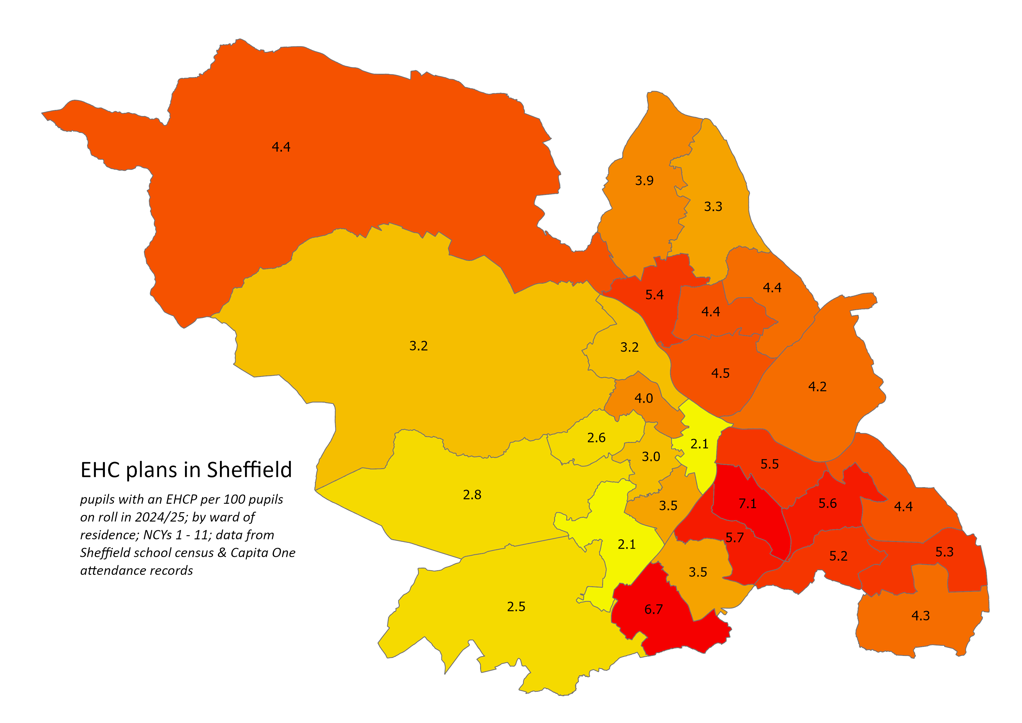#### Sen Support {.unnumbered}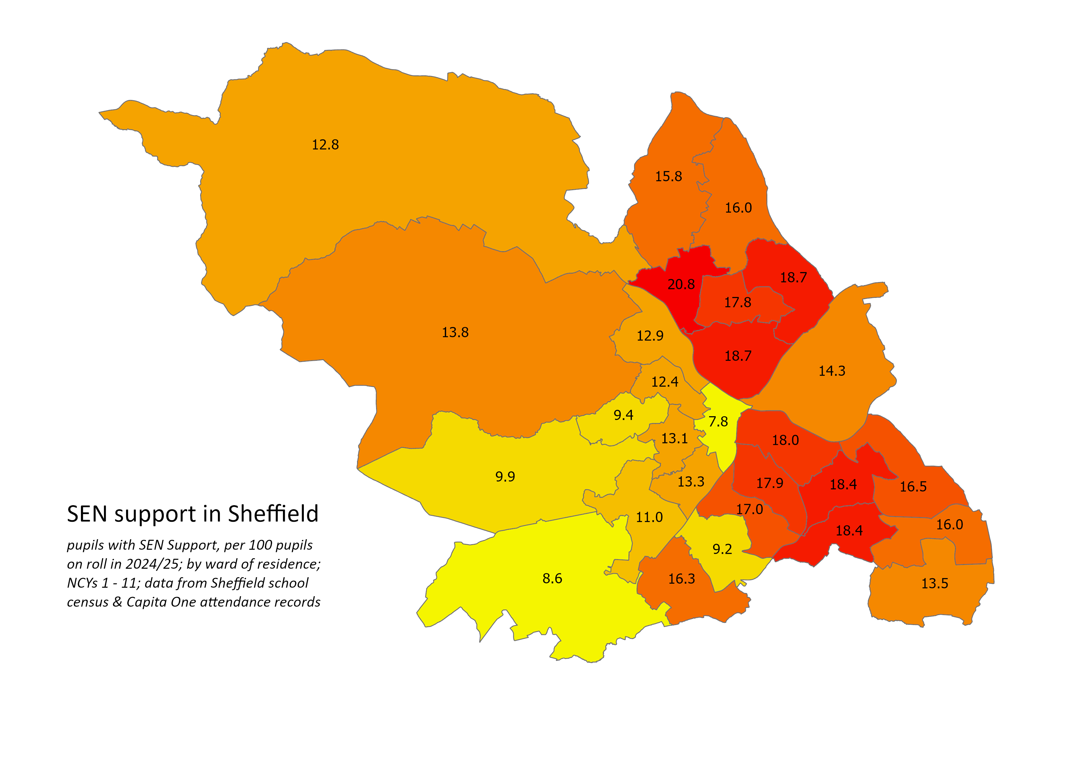#### Speech, Language & Communication Needs {.unnumbered}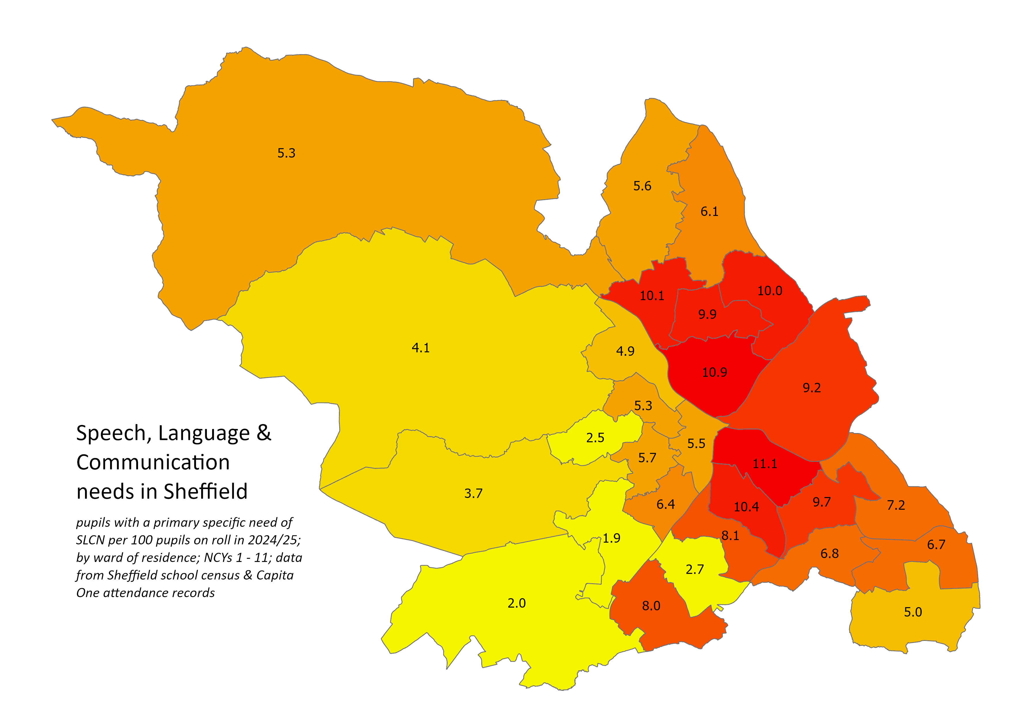#### Social, Emotional & Mental Health Needs {.unnumbered}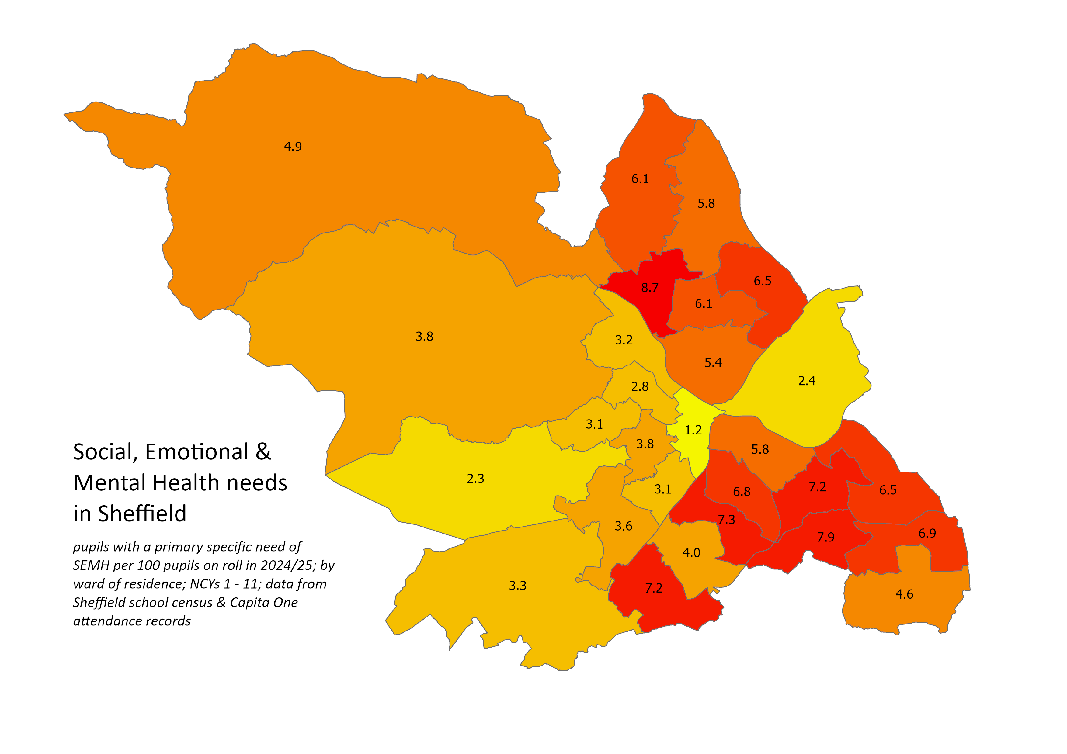#### Autism {.unnumbered}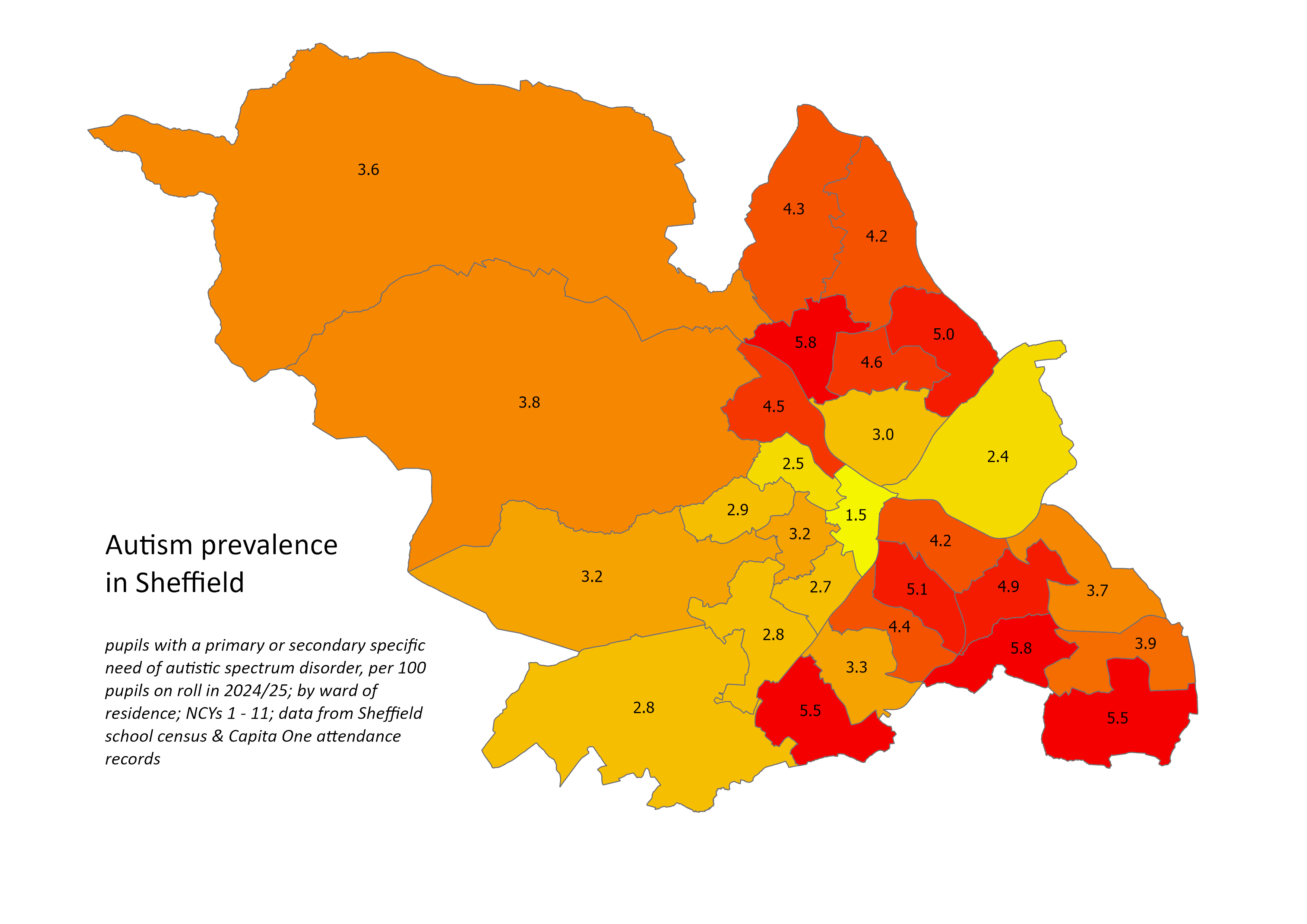#### Physical disabilities {.unnumbered}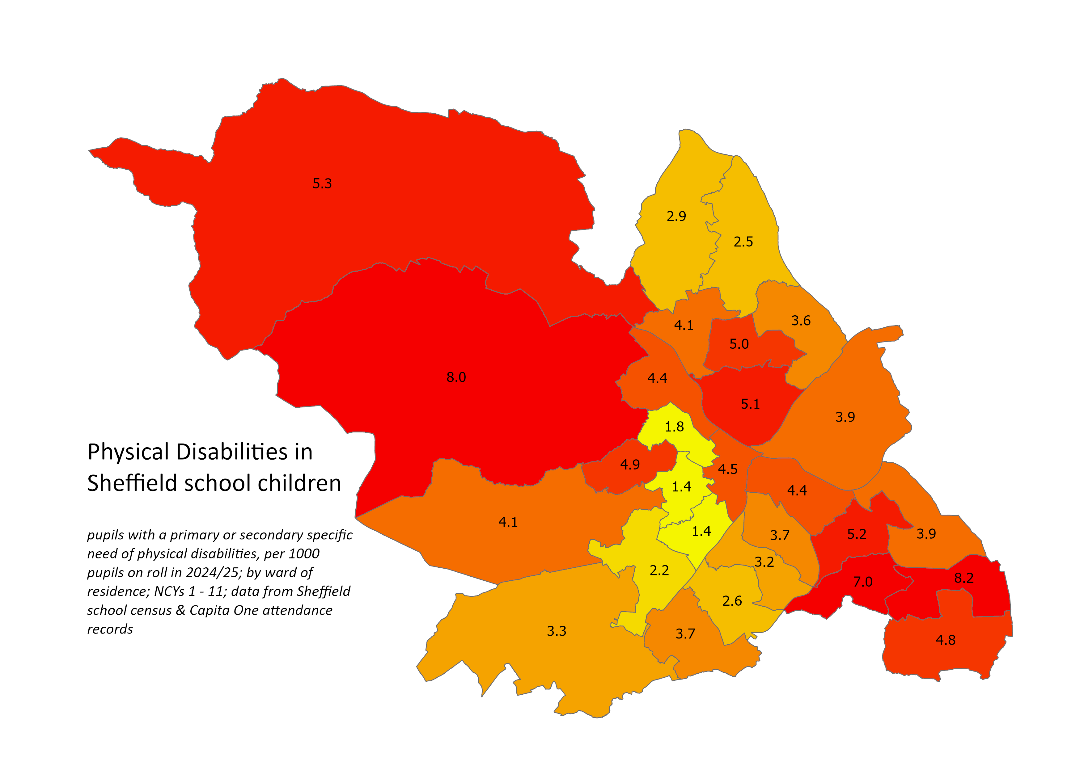#### Learning Difficulties {.unnumbered}::: callout-noteThe map below shows the prevalence of all learning difficulties listed in the school census data: moderate, specific, severe, and profound & multiple.:::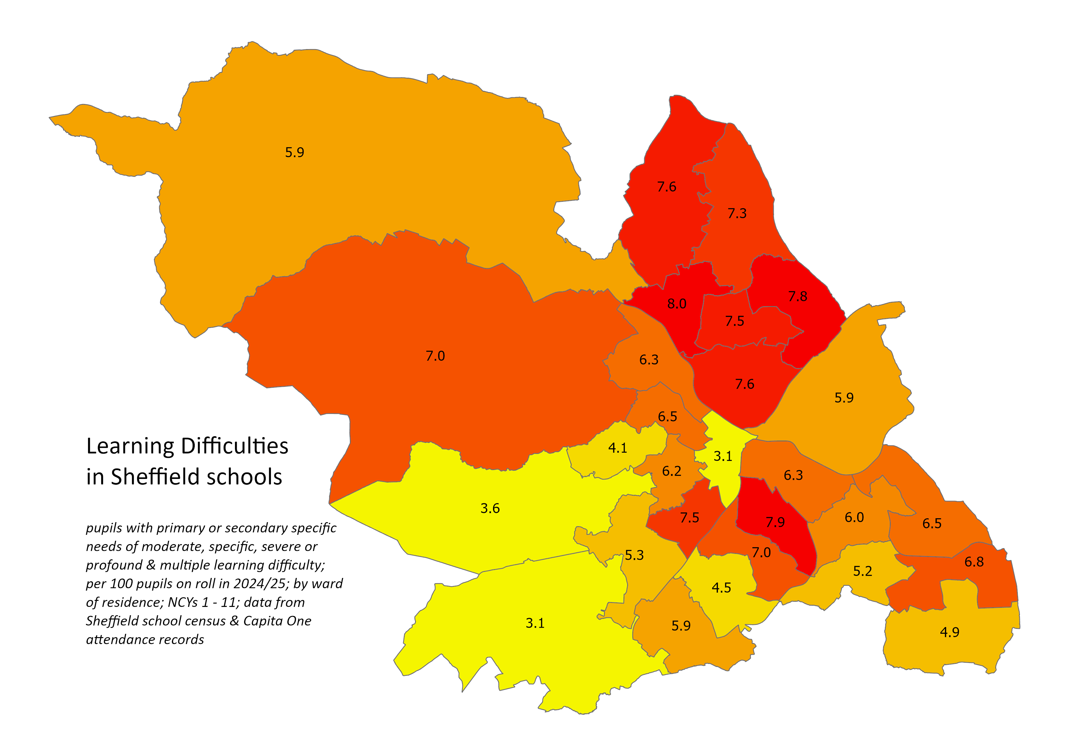#### Visual Impairment {.unnumbered}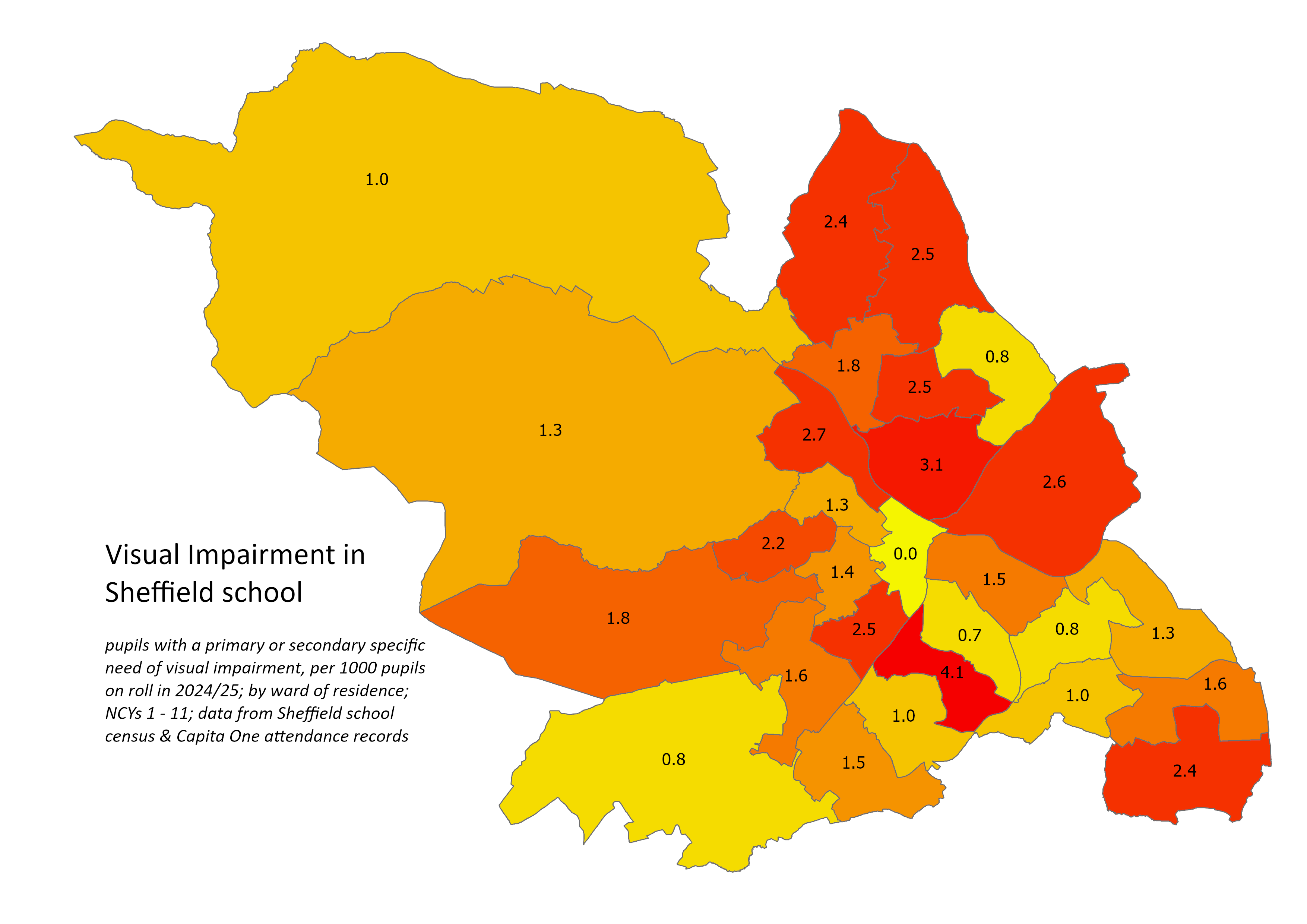#### Hearing impairment {.unnumbered}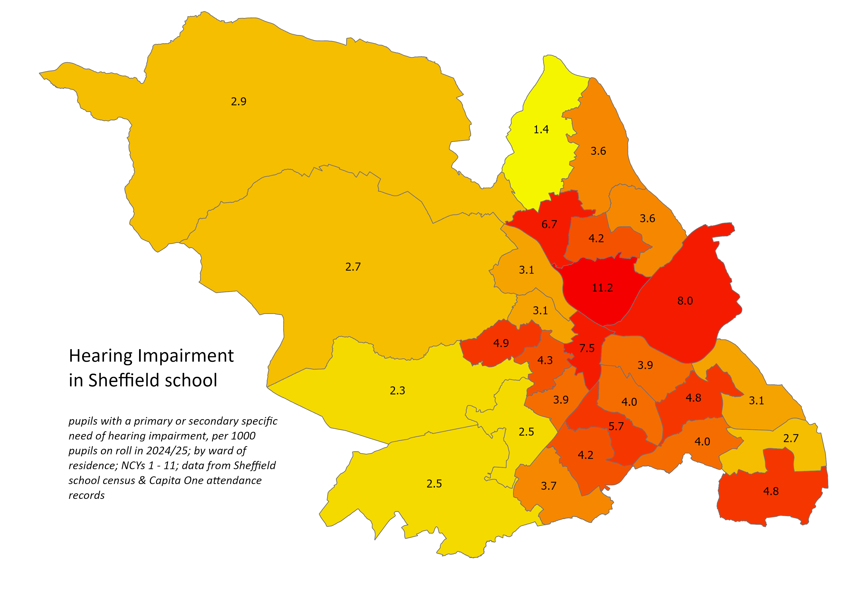#### Multi-sensory impairment {.unnumbered}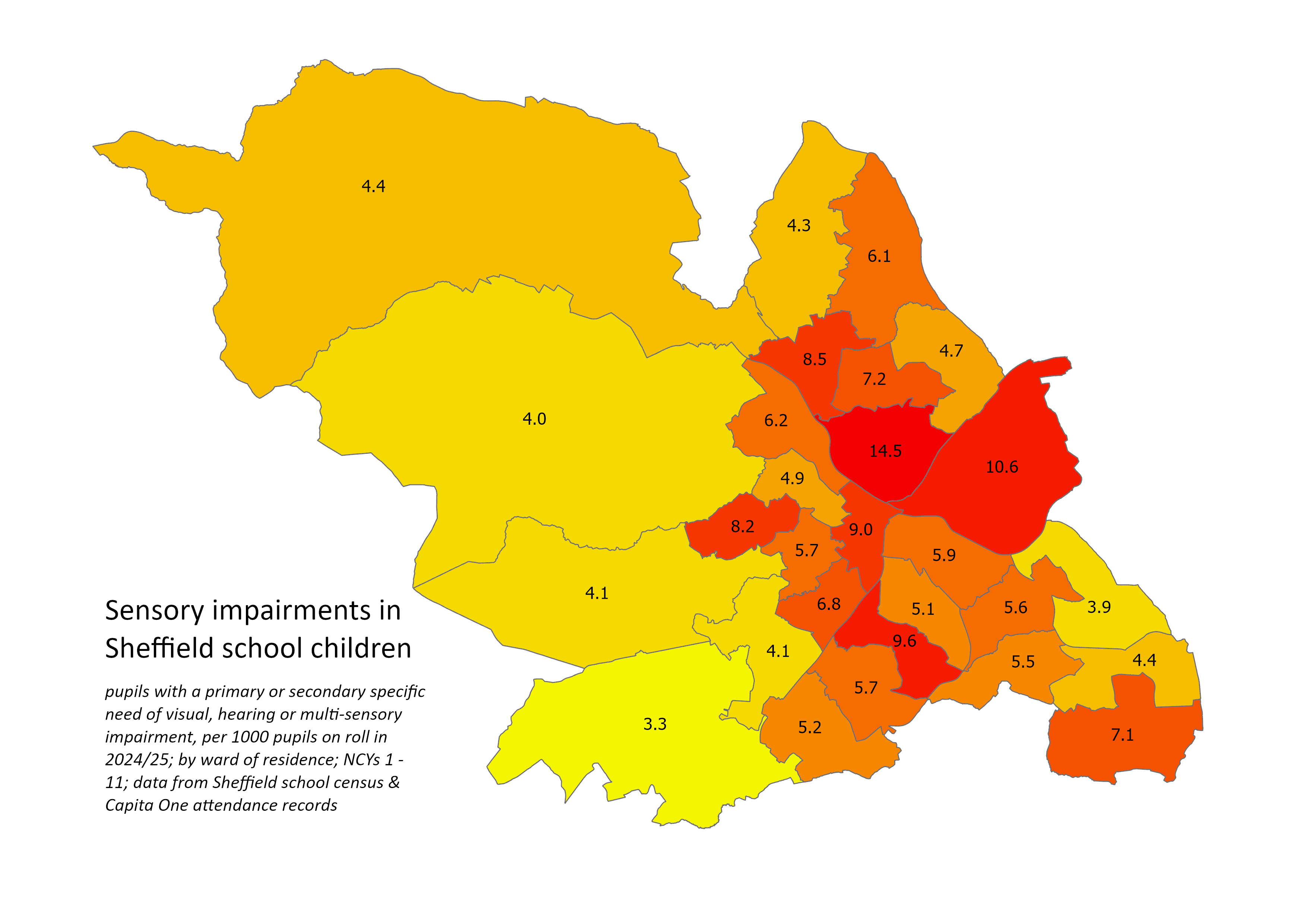## DeprivationMeasures of deprivation correlate strongly with the prevalence of special educational needs, more so for SEN support, and less so for pupils with an EHCP.::: callout-cautionThe apparent prevalences seen here probably result from differences in the true prevalences of SEN in the population, but may also reflect differences in engagement with the system, recording or policy. It is difficult to quantify the relative contributions of these factors from the data, though discussion of these issues with teachers, SEN workers and others on the front line may provide insight.:::Some wards seem to have lower SEN levels than might be expected from their deprivation measures alone, and appear *below* the main groupings on these charts - most noteably Darnall, Burngreave and Firth Park. Other wards appear to have higher prevalence than expected from deprivation measures alone, appearing *above* the main groupings: e.g. Birley, Beighton, Park & Arbourthorne.Note that due to it's low population, city ward is often an outlier on plots such as these.```{r}#| label: plot sen support by wardggplot( ward_sen_summary,aes(x = ward_imd_score, y = sen_support_pc *0.01 )) +geom_point() +geom_text_repel(aes(label = ward), size =2.5,segment.colour ="gray") +#geom_smooth(method = "lm") +scale_y_continuous(labels = scales::percent) +labs(title ="SEN support prevalence by ward level deprivation score", subtitle ="% of pupils on roll in 2024-25 with SEN support, by ward of residence",caption ="attendance data from Capita One",y ="% of pupils with sen support",x ="Indices of multiple deprivation score (2019)")``````{r}#| label: plot ehcp prevalence by wardggplot( ward_sen_summary,aes(x = ward_imd_score, y = ehcp_pc *0.01 )) +geom_point() +geom_text_repel(aes(label = ward), size =2.5,segment.colour ="gray") +#geom_smooth(method = "lm") +scale_y_continuous(labels = scales::percent) +labs(title ="EHCP prevalence by ward level deprivation score", subtitle ="% of pupils on roll in 2024-25 with an EHCP, by ward of residence",caption ="data from Capita One",y ="% of pupils with an EHCP",x ="Indices of multiple deprivation score (2019)")```The relationship between deprivation and speech, language & communication needs is particularly strong.```{r}#| label: plot slcn prevalence by wardggplot( ward_sen_summary,aes(x = ward_imd_score, y = slcn_pc *0.01 )) +geom_point() +geom_text_repel(aes(label = ward), size =2.5,segment.colour ="gray") +#geom_smooth(method = "lm") +scale_y_continuous(labels = scales::percent) +labs(title ="Speech, Language & Communication Needs prevalence by ward level deprivation score", subtitle ="% of pupils on roll in 2024-25 with a primary or secondary specific need of SLCN, by ward of residence",caption ="data from Capita One",y ="% of pupils with SLCN",x ="Indices of multiple deprivation score (2019)")```...and less pronounced for social, emotional & mental health needs, with some signficant outliers, particularly Darnall.```{r}#| label: plot semh prevalence by wardggplot( ward_sen_summary,aes(x = ward_imd_score, y = semh_pc *0.01 )) +geom_point() +geom_text_repel(aes(label = ward), size =2.5,segment.colour ="gray") +#geom_smooth(method = "lm") +scale_y_continuous(labels = scales::percent) +labs(title ="Social, Emotional & Mental Health needs prevalence by ward level deprivation score", subtitle ="% of pupils on roll in 2024-25 with a primary or secondary specific need of SEMH, by ward of residence",caption ="data from Capita One",y ="% of pupils with SEMH",x ="Indices of multiple deprivation score (2019)")```For autism, any link to deprivation is weak:```{r}#| label: plot autism prevalence by wardggplot( ward_sen_summary,aes(x = ward_imd_score, y = autism_pc *0.01 )) +geom_point() +geom_text_repel(aes(label = ward), size =2.5,segment.colour ="gray") +#geom_smooth(method = "lm") +scale_y_continuous(labels = scales::percent) +labs(title ="Autism prevalence by ward level deprivation score", subtitle ="% of pupils on roll in 2024-25 with a primary or secondary specific need of autistic spectrum disorder, by ward of residence",caption ="data from Capita One",y ="% of pupils with ASD",x ="Indices of multiple deprivation score (2019)")``````{r}#| label: plot pd prevalence by wardggplot( ward_sen_summary,aes(x = ward_imd_score, y = pd_pc *0.01 )) +geom_point() +geom_text_repel(aes(label = ward), size =2.5,segment.colour ="gray") +#geom_smooth(method = "lm") +scale_y_continuous(labels = scales::percent) +labs(title ="Physical Disabilities prevalence by ward level deprivation score", subtitle ="% of pupils on roll in 2024-25 with a primary or secondary specific need of autistic spectrum disorder, by ward of residence",caption ="data from Capita One",y ="% of pupils with PD",x ="Indices of multiple deprivation score (2019)")```## AttendanceOn average, school attendance is lower for children with SEN Support, and lower still for pupils with an EHC plan. These differences are greater in secondary schools than in primary, and the drop in attendance levels for SEN support children in secondary is particularly concerning.```{r}#| label: calculate attendance by SEN level#| message: FALSE#| fig-width: 4#| fig-height: 4sen_data <- attend |>filter(year ==2024, phase !="Nursery", phase !="6th form")# calculate average presence by term nameattend_sen <- sen_data |>summarise_attendance(grouping_vars =c("sen_level","phase","stud_id")) |>group_by(sen_level, phase) |>presence_mean_calc() # calculate overall averageattend_sen_overall <- sen_data |>summarise_attendance(grouping_vars =c("sen_level","phase","stud_id")) |>group_by(phase) |>presence_mean_calc() |>mutate(sen_level ="overall")attend_sen <-rbind(attend_sen, attend_sen_overall) |>mutate(fill_code =case_when(sen_level =='overall'~'total',TRUE~'others')) ``````{r}#| label: plot attendance by SEN level#| message: FALSE##| fig-width: 6##| fig-height: 5# plotggplot(attend_sen, aes(x =reorder(sen_level,mean.percent_present), y = mean.percent_present,fill = fill_code)) +geom_col(position =position_dodge(0.9), width =0.8)+geom_errorbar(aes(ymin = lower.ci.percent_present, ymax = upper.ci.percent_present), width =0.2, position =position_dodge(0.9))+geom_text(aes(label = scales::percent(round(mean.percent_present,3))), hjust =1, colour ="white", size =3, position =position_dodge(0.9)) +labs(title ="Attendance by SEN level",subtitle ="Average % of sessions attended in 2023/24 +- 95 CI",caption ="Attendance data from Capita One; SEN data from sheffield school census" )+ barplottheme_minimal +facet_grid(rows =vars(phase)) +coord_flip() +theme(axis.title.x = eb, axis.text.x = eb, legend.position ="none", strip.background = eb, plot.caption =element_text(size =7, face ="italic")) +scale_fill_manual(values =c("others"="#0072B2", "total"="#b47846"))```Plotting attendance over time by sen level shows how the attendance gap between primary and secondary age children widened after the pandemic. We can also see the gap widen between children with & without SEN. By 2024 an attendance gap of almost 10% had opened up between secondary age children with no SEN and those on SEN support; children with an EHCP plan were attending almost 12% lower. The post pandemic period saw a drop in attendance for all children, but the group with the biggest reduction was children in secondary schools who require SEN Support.::: callout-importantAt the time of writing, the last year has seen encouraging recovery in attendance for all groups shown here. The biggest improvements for those groups most heavily affected - secondary school pupils on SEN support or with EHCP plans.:::```{r}#| label: plot attendance over time by sen level and phase#| warning: false##| fig-width: 10##| fig-height: 8plot_data <- attend_year_sen_level_sch_census_phase |>mutate(sen_level =fct_relevel(sen_level,c("No SEN","SEN Support", "EHCP")),phase =fct_relevel(school_ed_phase_corrected,c("Nursery","Primary","Secondary","6th form")) ) |>filter(phase %in%c("Primary","Secondary"),!is.na(sen_level), year >=2018)ggplot(plot_data, aes(x = year, y = percent_present, colour = school_ed_phase_corrected)) +geom_point() +geom_line(linetype ="dashed", alpha =0.5) +geom_text(data = plot_data |>filter(phase =="Primary"),aes(label = scales::percent(percent_present, accuracy =0.1L)), size =2.5, vjust =-0.5) +geom_text(data = plot_data |>filter(phase =="Secondary"),aes(label = scales::percent(percent_present, accuracy =0.1L)), size =2.5, vjust =1.2) + barplottheme_minimal +scale_y_continuous(labels = scales::percent) +#, limits = c(0.7,1)) +scale_x_continuous(breaks =seq(2018,2025)) +labs(title ="Overall attendance by academic year and SEN level in <b><span style='color:#dd5129'>primary </span></b>and <b><span style='color:#0f7ba2;'>secondary</b></span> schools",subtitle ="percentage of sessions missed per year; all Sheffield pupils; 2025 data is part year",caption ="attendance data from Capita One") +theme(plot.title =element_markdown(size =12),legend.position ="none",axis.title.x = eb, axis.title.y = eb, axis.text.y = eb,strip.background = eb,panel.spacing =unit(2, "lines") ) + MetBrewer::scale_fill_met_d("Egypt") +facet_grid(rows =vars(sen_level), scales ="free_y") +coord_cartesian(clip ="off")```Plotting attendance by national curriculum year and SEN level produces three profiles of attendance. Here we see that the transition to secondary school has the most severe impact on attendance for children requiring SEN support. And while all children see a decline in average attendance through secondary, the decline is more severe for children requiring SEN support. Pupils with an EHC plan show a steady decline from NCY 3 onwards, and no discernable step down into secondary.```{r}attend_sen_level_ncy <- attend |>filter(year >=2018, ncy >=1, ncy <=11) |>group_by(sen_level, ncy) |>summarise_avg() |>mutate(label =if_else(ncy ==max(ncy), sen_level, NA_character_))ggplot(attend_sen_level_ncy, aes(x = ncy, y = mean.percent_present,colour = sen_level, group = sen_level,label = label)) +geom_point() +geom_line() +geom_label_repel(hjust =0, nudge_y =c(0.05,0.02,0.02), min.segment.length =Inf, alpha =0.8) +geom_errorbar(aes(ymin = lower.ci.percent_present, ymax = upper.ci.percent_present), width =0.2, alpha =0.7)+scale_y_continuous(labels = scales::percent) +scale_x_continuous(breaks =seq(1,11)) +labs(title ="Attendance by SEN level and national curriculum year",subtitle ="Average % of sessions attended since 2018 +-95CI",caption ="Attendance data from Capita One; SEN data from sheffield school census" ) +theme(axis.title.y = eb, legend.position ="none") +geom_vline(aes(xintercept =6.5), linetype ="dotted", colour ="gray70", size =1.2) +annotate("text", label ="primary", y =0.99, x =3.5, colour ="gray40") +annotate("text", label ="secondary", y =0.99, x =9, colour ="gray40")```## AttainmentAttainment data is available by SEN level and local authority from the DfE. Here we look at how attainment at Key Stage 2 (KS2) and Key Stage 4 (KS4) differs by SEN status, how Sheffield compares with the core cities, and how this is changing over time. There are many different measures of attainment in the published data, but here we focus on two: - At KS2, the % of pupils meeting expected standard in reading, writing and maths. - At KS4, the average *attainment 8* score, which measures attainment across a pupil's eight best subjects.At both KS2 and KS4, children with SEN support have lower attainment than those no SEN, and children with EHC plans have lower attainment still.```{r}#| label: plot ks2 attainment by SEN status Sheffield#| fig-height: 3ks2_att |>filter(sheffield_flag ==1, year ==max(year), breakdown_topic =="SEN status", gender =="Total",!breakdown %in%c("All SEN","SEN unclassified") ) |>mutate(sen_level =fct_relevel(breakdown, c("No SEN","SEN support","EHC plan"))) |>select(la_name, sen_level, pt_rwm_met_expected_standard) |>ggplot(aes(x =reorder(sen_level,pt_rwm_met_expected_standard),y = pt_rwm_met_expected_standard,label = pt_rwm_met_expected_standard) ) +geom_col(fill ="steel blue", width =0.8) +geom_text(colour ="white", size =4, hjust =1.5) +labs(title ="Key Stage 2 attainment in Sheffield by SEN level",subtitle ="% of pupils meeting expected standard in reading, writing & maths; 2023",caption ="data from DfE") +coord_flip() + barplottheme_minimal +theme(axis.title = eb, axis.text.x = eb, legend.position ="none")``````{r}#| label: plot ks4 attainment by SEN status Sheffield#| fig-height: 3ks4_att |>filter(sheffield_flag ==1, time_period ==max(time_period), breakdown =="SEN status", gender =="Total") |>mutate(sen_status =fct_recode(sen_status,"EHC plan"="SEN State EHC", "SEN support"="SEN Supp")) |>mutate(sen_level =fct_relevel(sen_status, c("No SEN","SEN support","EHC plan"))) |>select(time_period, la_name, sen_level, avg_att8) |>ggplot(aes(x =reorder(sen_level,avg_att8, desc =TRUE),y = avg_att8,label = avg_att8) ) +geom_col(fill ="steel blue", width =0.8) +geom_text(colour ="white", size =4, hjust =1.5) +labs(title ="Key Stage 4 attainment in Sheffield by SEN level",subtitle ="Average attainment 8 score of all pupils; 2023",caption ="data from DfE") +coord_flip() + barplottheme_minimal +theme(axis.title = eb, axis.text.x = eb, legend.position ="none")```Comparing with core cities, Sheffield shows similar performance at KS2 to the average for SEN support and children with no SEN, but benchmarks poorly for children with an EHC plan. It's worth noting that there is large variation in the EHC plan attainment data here, that looks too great to be the result of local policy alone.```{r}#| label: plot ks2 attainment core cities comparison#| fig-height: 6ks2_att |>filter(core_city_flag ==1, year ==max(year), breakdown_topic =="SEN status", gender =="Total",!breakdown %in%c("All SEN","SEN unclassified") ) |>mutate(sen_level =fct_relevel(breakdown, c("No SEN","SEN support","EHC plan")),fill_code =case_when(la_name =='Sheffield'~'Sheffield', la_name =='core cities average'~'core cities average',TRUE~'others')) |>select(year, la_name, sen_level, pt_rwm_met_expected_standard, fill_code) |>ggplot(aes(x =reorder_within(la_name,pt_rwm_met_expected_standard, within = sen_level),y = pt_rwm_met_expected_standard *0.01,fill = fill_code) ) +geom_col(position ="dodge") +facet_grid(rows =vars(sen_level), scales ="free") +coord_flip() +scale_x_reordered() +scale_y_continuous(labels = scales::percent) +labs(title ="Key Stage 2 attainment by SEN level - core cities",subtitle ="Percentage of pupils meeting the expected standard in reading, writing and maths (combined); 2023",y ="% of pupils meeting expected standard",caption ="data from DfE") + barplottheme_minimal +theme(legend.position ="none", axis.title.y = eb, strip.background = eb,axis.text.y =element_text(size =7.5), strip.text =element_text(size=10)) +scale_fill_manual(values =c("others"="#0072B2", "Sheffield"="#b47846", "core cities average"="#00a3ff"))```At KS4, Sheffield benchmarks around the average for children with an EHC plan, but poorly for those with SEN support.```{r}#| label: plot ks4 attainment core cities comparison#| fig-height: 6ks4_att |>filter(core_city_flag ==1, year ==max(year), breakdown =="SEN status", gender =="Total") |>mutate(sen_status =fct_recode(sen_status,"EHC plan"="SEN State EHC", "SEN support"="SEN Supp")) |>mutate(sen_level =fct_relevel(sen_status, c("No SEN","SEN support","EHC plan"))) |>#select(la_name, sen_level, avg_att8) |> mutate(fill_code =case_when(la_name =='Sheffield'~'Sheffield', la_name =='core cities average'~'core cities average',TRUE~'others')) |>select(year, la_name, sen_level, avg_att8, fill_code) |>ggplot(aes(x =reorder_within(la_name,avg_att8, within = sen_level),y = avg_att8,fill = fill_code) ) +geom_col(position ="dodge") +facet_grid(rows =vars(sen_level), scales ="free") +coord_flip() +scale_x_reordered() +labs(title ="Key Stage 4 attainment by SEN level - core cities",subtitle ="Average attainment 8 score of all pupils; 2023",y ="Average attainment 8 score of all pupils",caption ="data from DfE") + barplottheme_minimal +theme(legend.position ="none", axis.title.y = eb, strip.background = eb,axis.text.y =element_text(size =7.5), strip.text =element_text(size=10)) +scale_fill_manual(values =c("others"="#0072B2", "Sheffield"="#b47846", "core cities average"="#00a3ff"))```For the years heavily affected by COVID, the DfE have not published the KS2 expected standard measure we used above, but the available data shows changes over time. Between 2019 and 2022 all children see a drop in attainment at KS2, and all see an improvement into 2023, but both SEN support and EHC plan children show a lesser drop to 2022 and a better recovery into 2023 than children with no SEN.```{r}#| label: plot ks2 attainment by SEN status over time Sheffield#| warning: false#| fig-height: 3ks2_att |>filter(sheffield_flag ==1,#year == max(year), breakdown_topic =="SEN status", gender =="Total",!breakdown %in%c("All SEN","SEN unclassified") ) |>mutate(label =if_else(year ==max(year), breakdown, NA_character_)) |>select(year, la_name, breakdown, pt_rwm_met_expected_standard, label) |>ggplot(aes(x = year,y = pt_rwm_met_expected_standard *0.01,colour = breakdown,group = breakdown,label = label) ) +geom_point() +geom_line() +#geom_text_repel(aes(label = pt_rwm_met_expected_standard), nudge_y = 2) +geom_label_repel(#nudge_x = 0.25, size =3,fontface ="bold",min.segment.length =Inf,hjust =1,alpha =0.75)+scale_y_continuous(labels = scales::percent) +labs(title ="Key Stage 2 attainment in Sheffield, over time & by SEN level",subtitle ="% of pupils meeting expected standard in reading, writing & maths",caption ="data from DfE; 2020 & 2021 data was not published") +theme(legend.position ="none", axis.title = eb, axis.line = eb, axis.ticks = eb) +coord_cartesian(clip ="off")```Finally on attainment, and at KS4 attainment peaking in 2021 and dropping slowly for all SEN groups.```{r}#| label: plot ks4 attainment by SEN status over time Sheffield#| warning: falseks4_att |>filter(sheffield_flag ==1, breakdown =="SEN status", gender =="Total") |>mutate(sen_level =fct_recode(sen_status,"EHC plan"="SEN State EHC", "SEN support"="SEN Supp")) |>select(year, la_name, sen_level, avg_att8) |>mutate(label =if_else(year ==max(year), sen_level, NA_character_)) |>select(year, la_name, sen_level, avg_att8, label) |>ggplot(aes(x = year,y = avg_att8,colour = sen_level,group = sen_level,label = label) ) +geom_point() +geom_line() +#geom_text_repel(aes(label = avg_att8), nudge_y = 1) +geom_label_repel(nudge_x =0.2, size =3,fontface ="bold",min.segment.length =Inf) +labs(title ="Key Stage 4 attainment in Sheffield, over time & by SEN level",subtitle ="Average attainment 8 score of all pupils",y ="Average attainment 8 score of all pupils",caption ="data from DfE") +theme(legend.position ="none", axis.title = eb, axis.line = eb, axis.ticks = eb)```## ExclusionsExclusion rates remain very low in primary schools, but rates are consistently higher for SEN support pupils. There has also been a recent rise in fixed period exclusions for primary aged children with an EHC plan.```{r}#| label: calculate exclusion volumes and rates by sen level#| warning: false#| message: false# calculate exclusion ratesexcl_sen_level_phase_yr <- exclusion |>rename(year = exam_year) |>filter(!is.na(year),!phase %in%c("Nursery", "6th form")) |>mutate(sen_level =replace_na(sen_level,"No SEN")) |>filter(!excl_category_description %in%c("Lunchtime Only Exclusion","Reinstated from Permanent","Reinstated from Fixed Period","Reinstated from Suspension"),!is.na(excl_category_description)) |>#select(year, sen_level, excl_category_description, phase) |>group_by(year, sen_level, excl_category_description, phase) |>tally(n ="exclusion_count") |>ungroup() |>complete(year, sen_level, excl_category_description, phase, fill=list(exclusion_count=0))# calculate totalstotals_sen_level_phase_yr <- attend |>group_by(sen_level, phase, year) |>summarise(pupil_count =n_distinct(stud_id))# join totals excl_sen_level_phase_yr <- excl_sen_level_phase_yr |>filter(!excl_category_description %in%c("Reinstated from Permanent","Reinstated from Fixed Period")) |>left_join(totals_sen_level_phase_yr, by =c("sen_level","phase","year")) |>mutate(exclusions_per_10k = exclusion_count / (pupil_count /10000)) |>#rename(`SEN level` = sen_level) |> filter(!phase %in%c("Nursery", "6th form")) |>filter(year <2025) |>## REMOVE THIS LINE ONCE THE COMPLETE 2024 data is availablemutate(label =if_else(year ==max(year), sen_level, NA_character_))``````{r}#| label: plot exclusion rates over time primary#| warning: false#| message: falseggplot(excl_sen_level_phase_yr |>filter(phase =="Primary"),aes(x = year, colour = sen_level,group = sen_level,y = exclusions_per_10k)) +geom_point() +geom_line() +geom_label_repel(aes(label = label),min.segment.length =Inf,max.overlaps =Inf,nudge_x =0.5,hjust =1,size =3,fontface ="bold",na.rm =TRUE) +facet_wrap(vars(excl_category_description), nrow =2,scales ="free_y") +labs(title ="Exclusion rates by SEN level - Sheffield primary schools",subtitle ="fixed and permanent exclusions per 10,000 pupils per year",caption ="exclusion data from Capita One; SEN data from sheffield school census") +scale_x_continuous(limits =c(2016,2027), breaks =seq(2006,2024)) +theme(legend.title = eb,axis.title = eb,strip.background = eb,strip.placement ="top",axis.text.x =element_text(size =6.5),legend.position ="none")```Exclusion rates in Secondary are rising dramatically both for pupils with no SEN, and those with SEN support (where, just as in primary, rates have always been higher), though not for those with an EHC plan.```{r}#| label: plot exclusion rates over time secondary#| warning: false#| message: falseggplot(excl_sen_level_phase_yr |>filter(phase =="Secondary"),aes(x = year, colour = sen_level,group = sen_level,y = exclusions_per_10k)) +geom_point() +geom_line() +geom_label_repel(aes(label = label),min.segment.length =Inf,max.overlaps =Inf,nudge_x =0.5,hjust =1,size =3,fontface ="bold",na.rm =TRUE) +facet_wrap(vars(excl_category_description), nrow =2,scales ="free_y") +labs(title ="Exclusion rates by SEN level - Sheffield secondary schools",subtitle ="fixed and permanent exclusions per 10,000 pupils per year",caption ="exclusion data from Capita One; SEN data from sheffield school census") +scale_x_continuous(limits =c(2016,2027), breaks =seq(2006,2024)) +theme(legend.title = eb,axis.title = eb,strip.background = eb,strip.placement ="top",axis.text.x =element_text(size =6.5),legend.position ="none")```The above charts show the rates per 10,000 pupils, so for completion here we include a table of the underlying numbers for 2023/24:```{r}#| label: table of exclusion rates#| warning: false#| message: false# calculate exclusion ratesexcl_sen_level_phase <- exclusion |>mutate(sen_level =replace_na(sen_level,"No SEN")) |>filter(exam_year ==2023, excl_category_description !="Lunchtime Only Exclusion") |>group_by(exam_year, sen_level, excl_category_description, phase) |>tally(n ="exclusion_count") |>ungroup() |>select(-exam_year)# calculate totalstotal_23 <- attend |>filter(year ==2023) |>group_by(sen_level, phase) |>summarise(pupil_count =n_distinct(stud_id))# join totals excl_sen_level_phase <- excl_sen_level_phase |>filter(excl_category_description !="Reinstated from Permanent") |>left_join(total_23, by =c("sen_level","phase")) |>mutate(exclusions_per_10k = exclusion_count / (pupil_count /10000)) |>#rename(`SEN level` = sen_level) |> filter(!phase %in%c("Nursery", "6th form"))# pivot wider by school phaseexcl_sen_level_phase_table <- excl_sen_level_phase |>pivot_wider(names_from ="phase",values_from =c("exclusion_count","pupil_count","exclusions_per_10k") ) |>relocate(contains("Primary"), .before =contains("Secondary"))# display the table:excl_sen_level_phase_table |>group_by(sen_level) |>gt(rowname_col ="excl_category_description") |>tab_spanner(id =1, label ="primary", columns = dplyr::contains("Primary")) |>tab_spanner(id =2, label ="secondary", columns = dplyr::contains("Secondary")) |>#tab_spanner(id = 3, label = "No SEN", rows = dplyr::contains("No SEN")) |> cols_label(contains("pupil_count") ~"pupils on roll",contains("exclusion_count") ~"exclusions",contains("per_10k") ~"exclusions per 10,000 pupils", excl_category_description ~"exclusion type" ) |>#tab_row_group(rows = sen_level,# label = "SEN level") |> tab_header(title ="Exclusion rates in Sheffield by SEN level and school phase",subtitle ="counts of exclusions and pupils on roll in 2023/24; data from School Census & Capita One attendance records") |>tab_options(table.align ="left",table.font.size =10,row_group.font.size =12,row_group.padding.horizontal =-20,heading.title.font.size =12,heading.subtitle.font.size=10,heading.align ="left",column_labels.font.size =10,stub.font.size =10 ) |>cols_align("left",'excl_category_description' ) |>fmt_number(columns =contains("per_10k"),#n_sigfig = 3,use_seps =FALSE,decimals =1) |>sub_missing(missing_text ="-")```## Distance to schoolChildren with SEN may travel further to access a special school, or a more suitable school. We calculated the straight line distance between home and school postcodes, in order to create the following distance profiles. Primary age children live closer to their school than secondary age children, with Over 40% of secondary age children with an EHC plan live over 5km from school.```{r}#| label: calculate and plot distance profiles by sen level primarydistance_by_sen_level <- sch_dist_sheff_23 |>rename(phase = school_ed_phase_corrected) |>filter(!is.na(sen_level), phase !="Nursery") |>#filter(school_ed_phase == "Primary") |> #left_join(stud_details_joined, by = "stud_id") |>#rename(sen_level = sen_level_attend) |> mutate(dist_bin =cut(dist_crow, breaks =c(-Inf,200,500,1000,2000,5000,10000,Inf))) |>group_by(dist_bin, sen_level, phase) |>summarise(child_count =n_distinct(stud_id))ggplot(distance_by_sen_level,aes(x = dist_bin,y = child_count,fill = sen_level,colour = sen_level,label = child_count)) +geom_col(position ="dodge") +geom_text(size =2.5, vjust =-0.5) +scale_x_discrete(labels =c("0-200m","200-500m","500m-1km","1-2km","2-5km","5-10km","10km+"))+facet_grid(rows =vars(sen_level), cols =vars(phase), scales ="free") +coord_cartesian(clip ="off") +labs(title ="Home to school distance for Sheffield pupils, by SEN level & phase",subtitle ="Count of pupils in 2023; straight line distance between home and school postcode",caption ="Data from Capita One attendance records and Sheffield school census") +theme(axis.title = eb, strip.background = eb, legend.position ="none", axis.text.y = eb, axis.line.y = eb, axis.ticks.y = eb,axis.text.x =element_text(size =7)) +scale_fill_brewer(palette ="Dark2") +scale_colour_brewer(palette ="Dark2")```
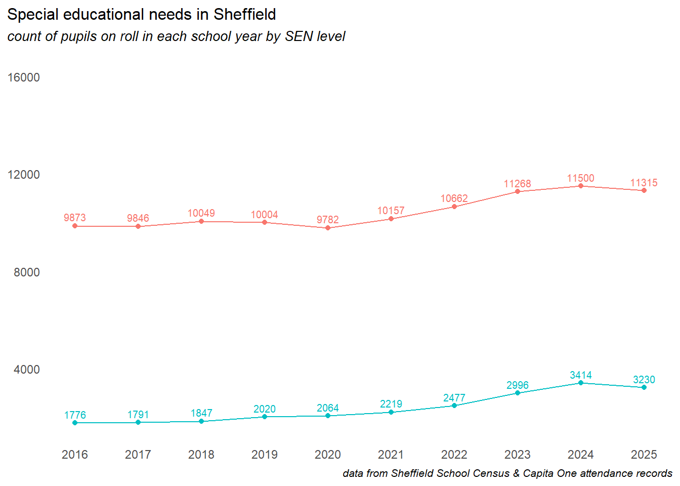
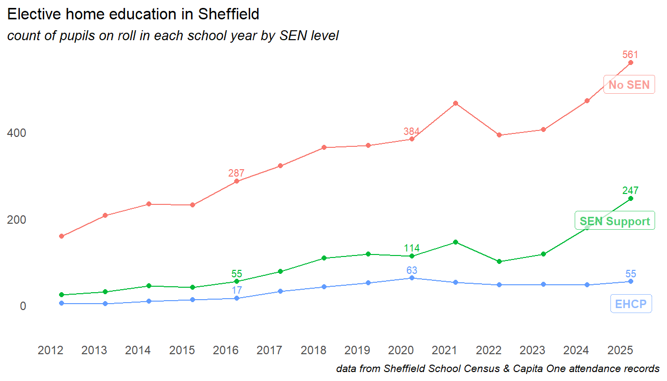
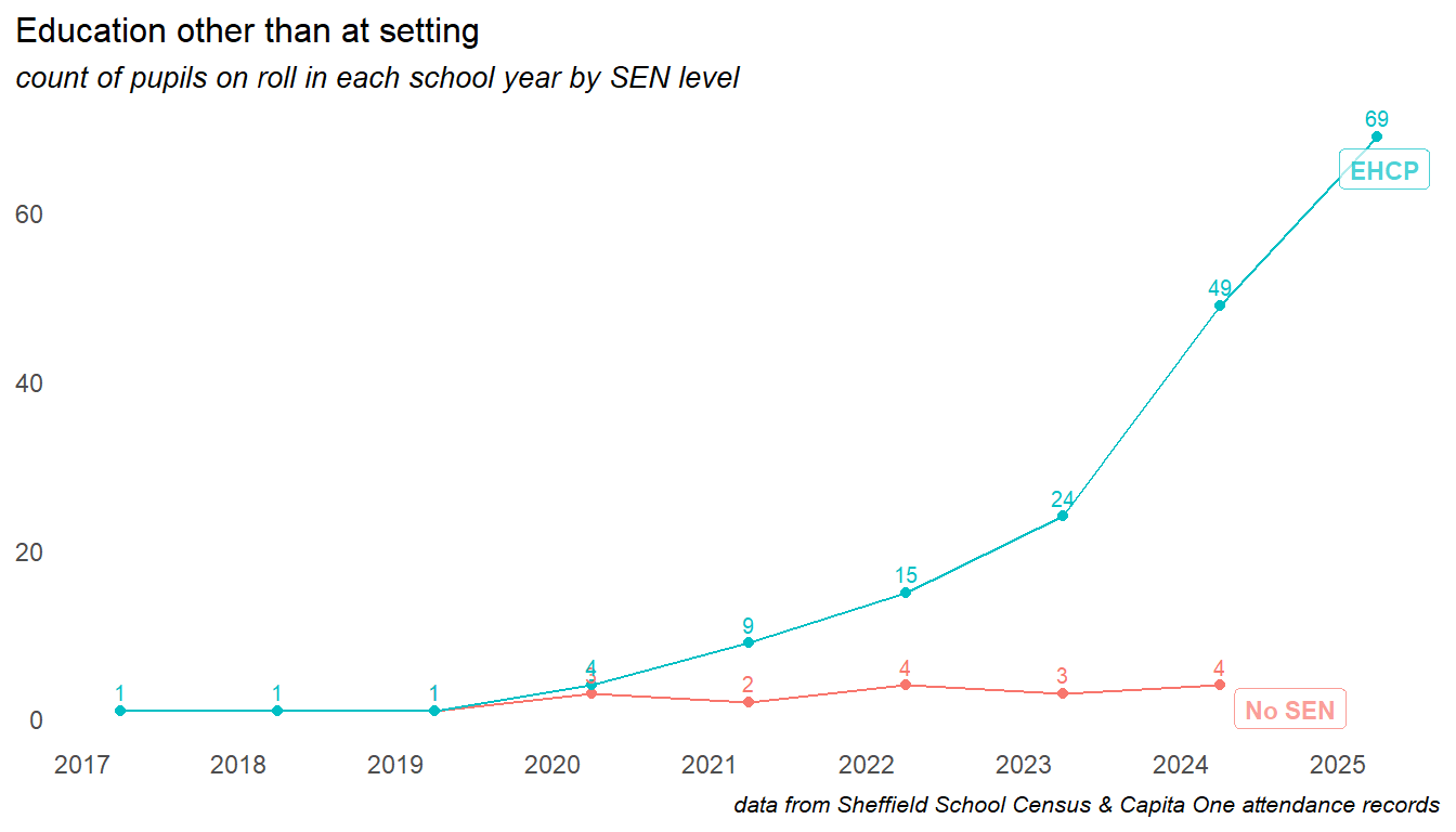
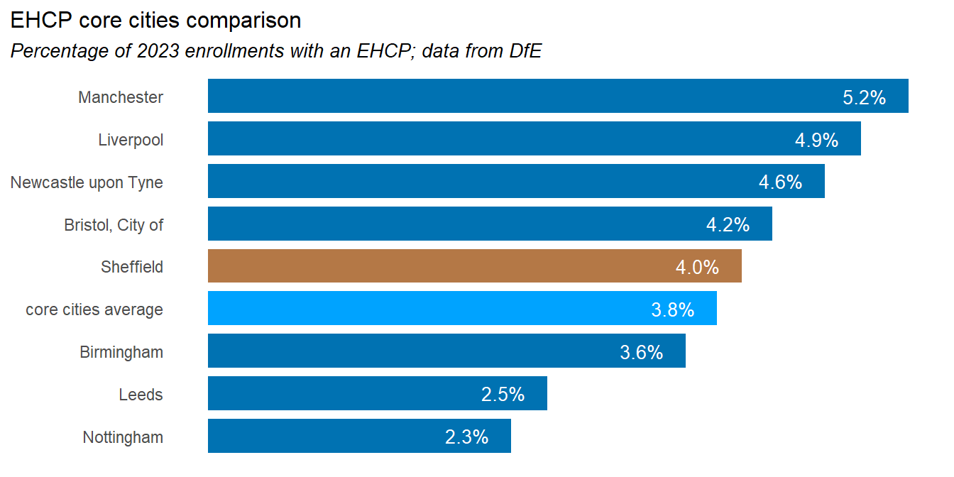
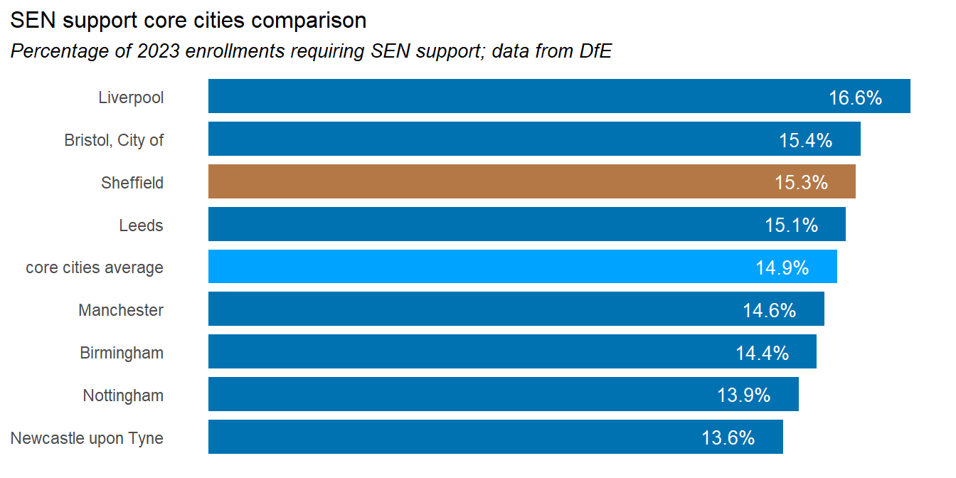
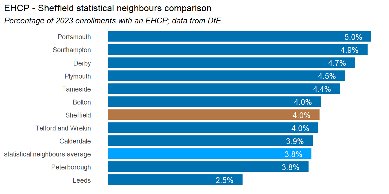
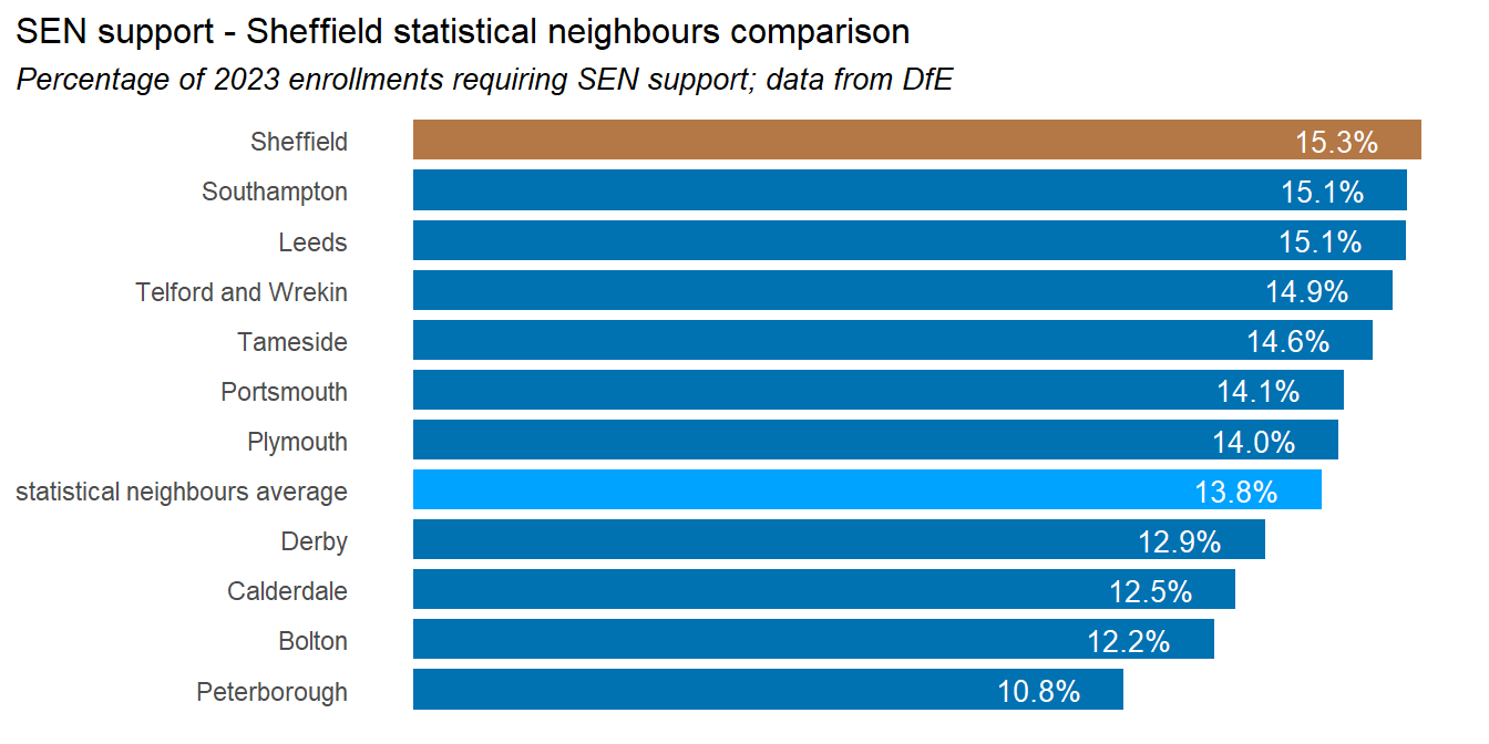
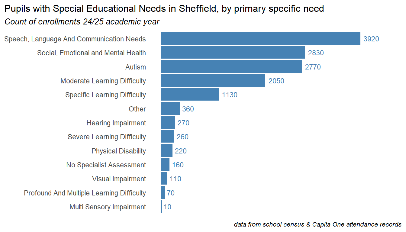
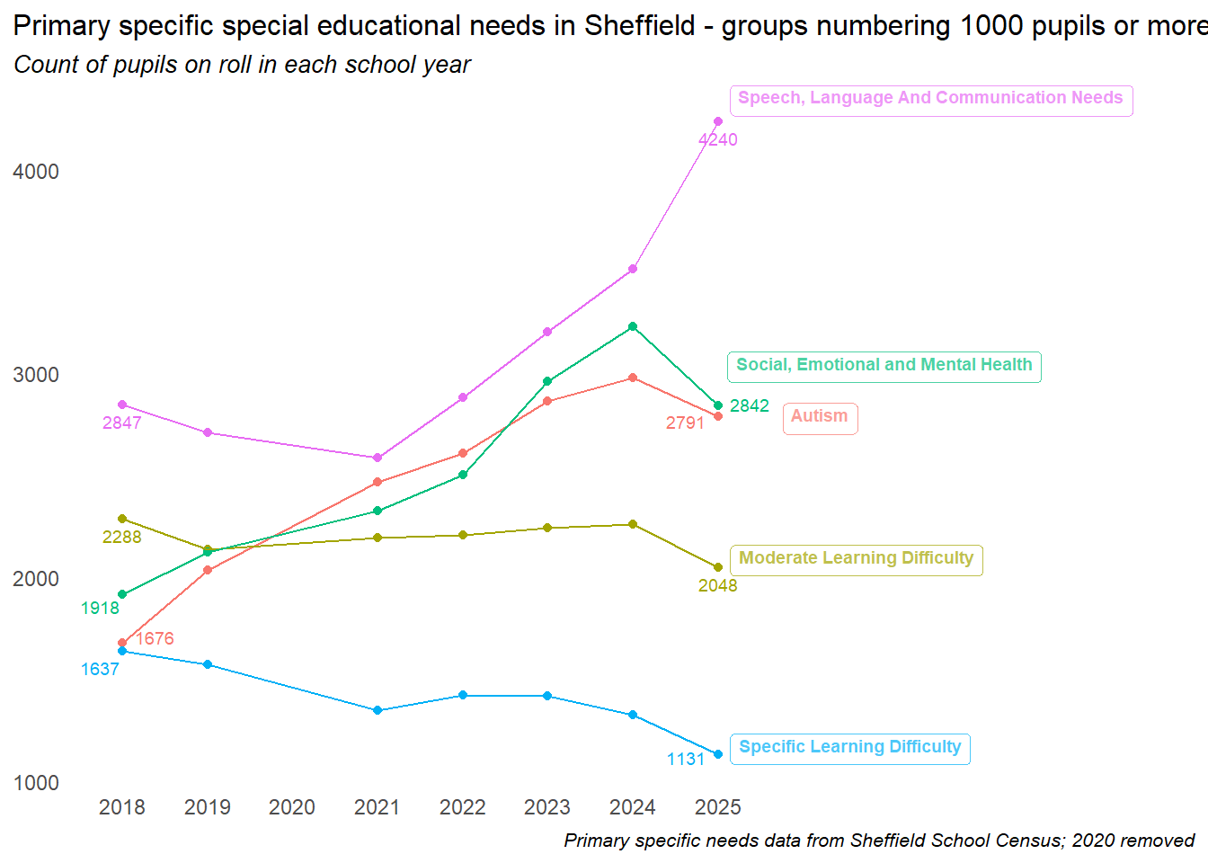
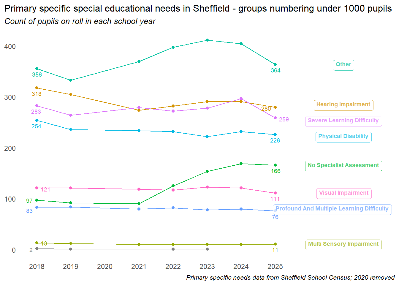
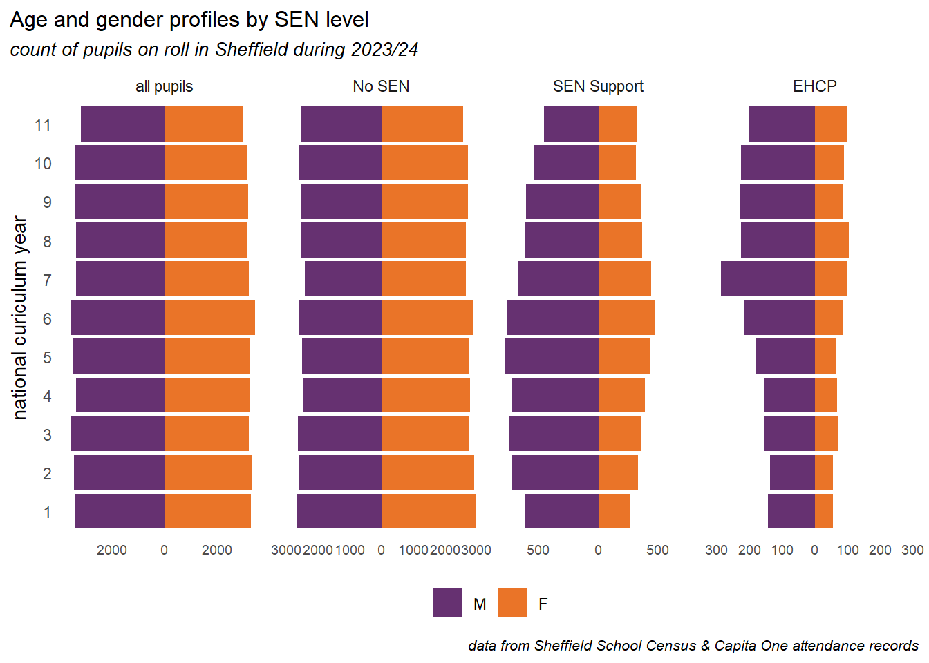
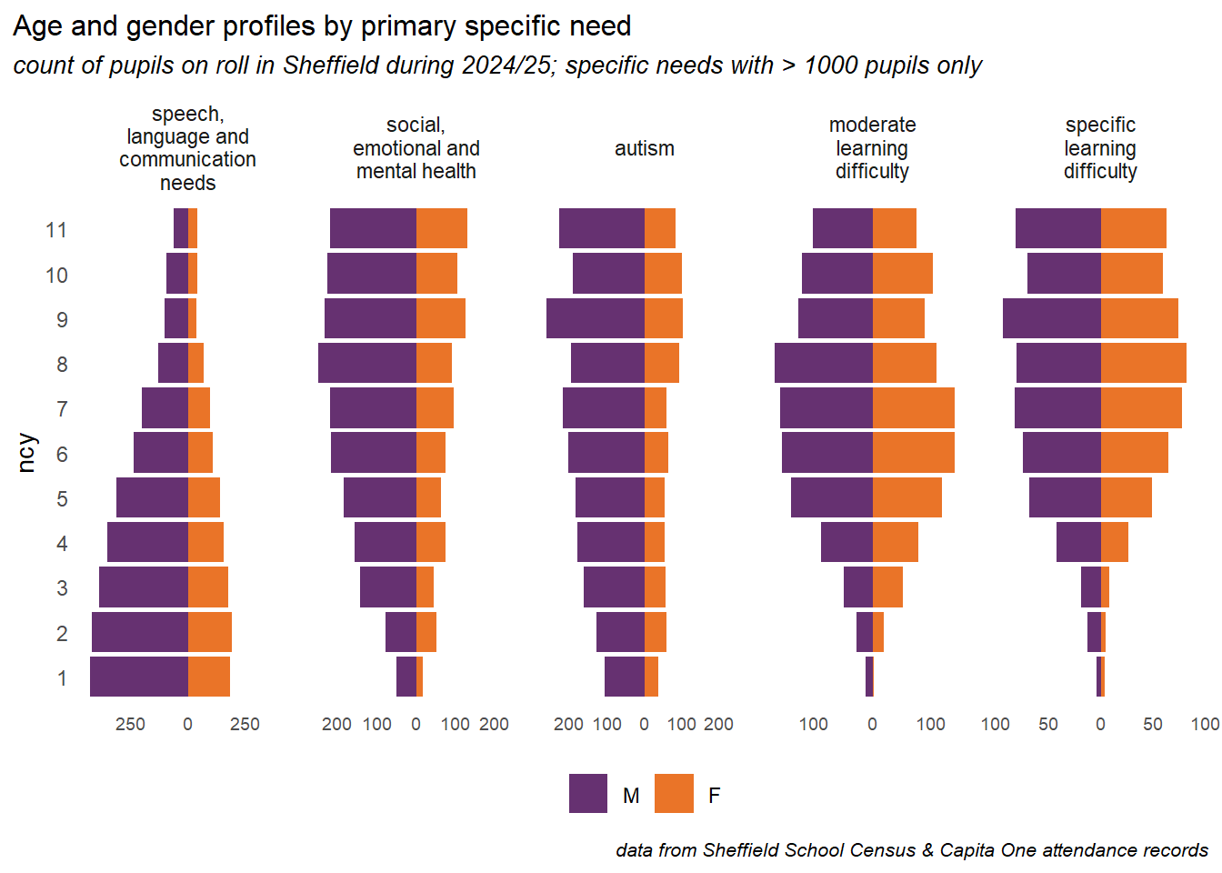
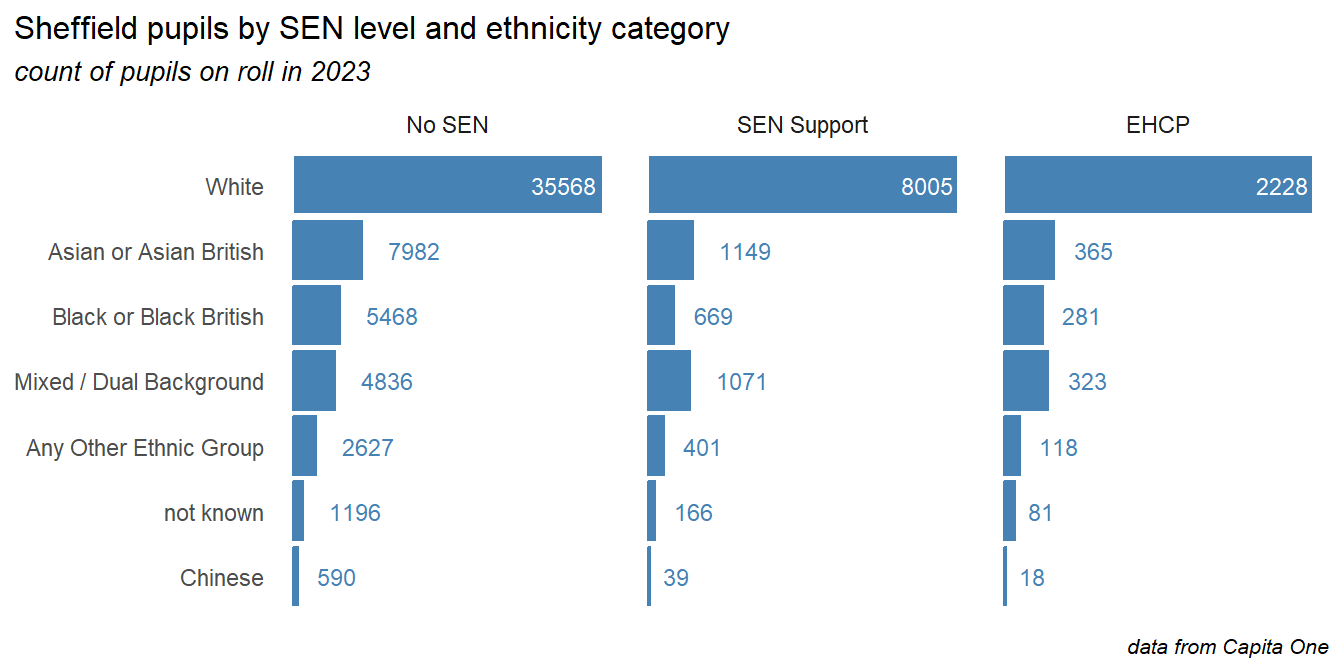
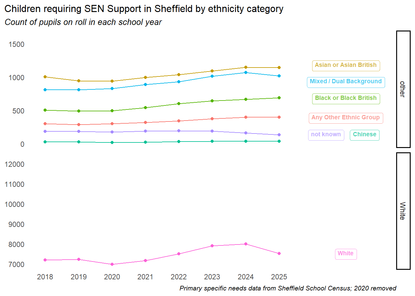
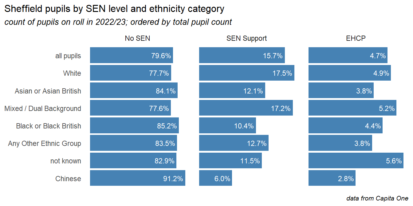


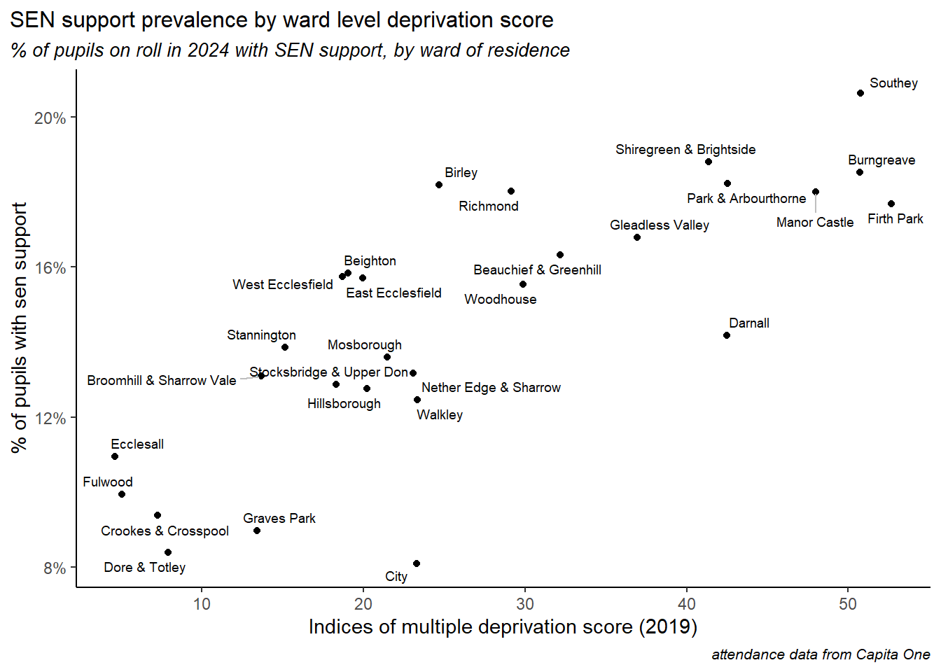
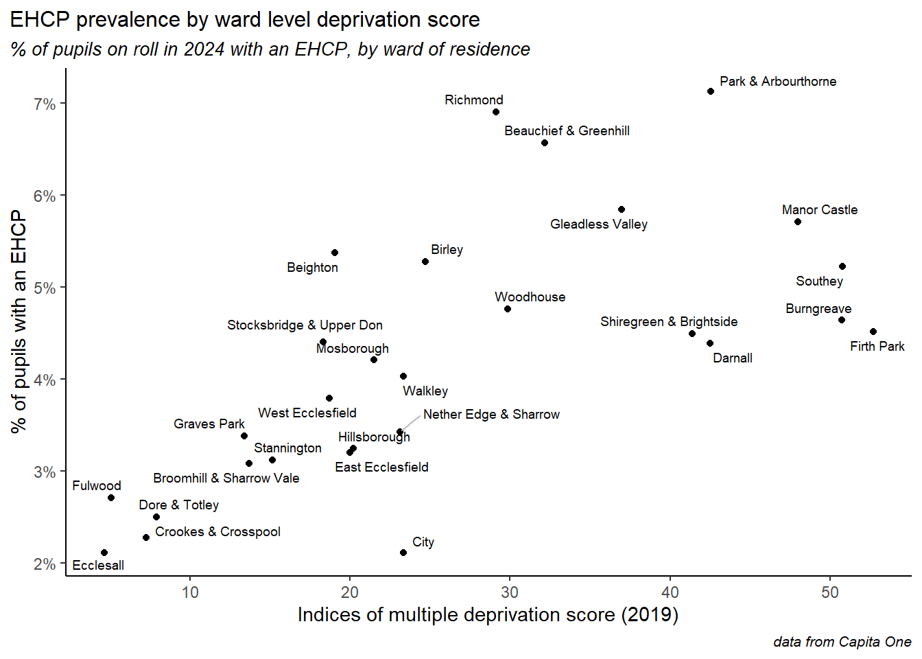
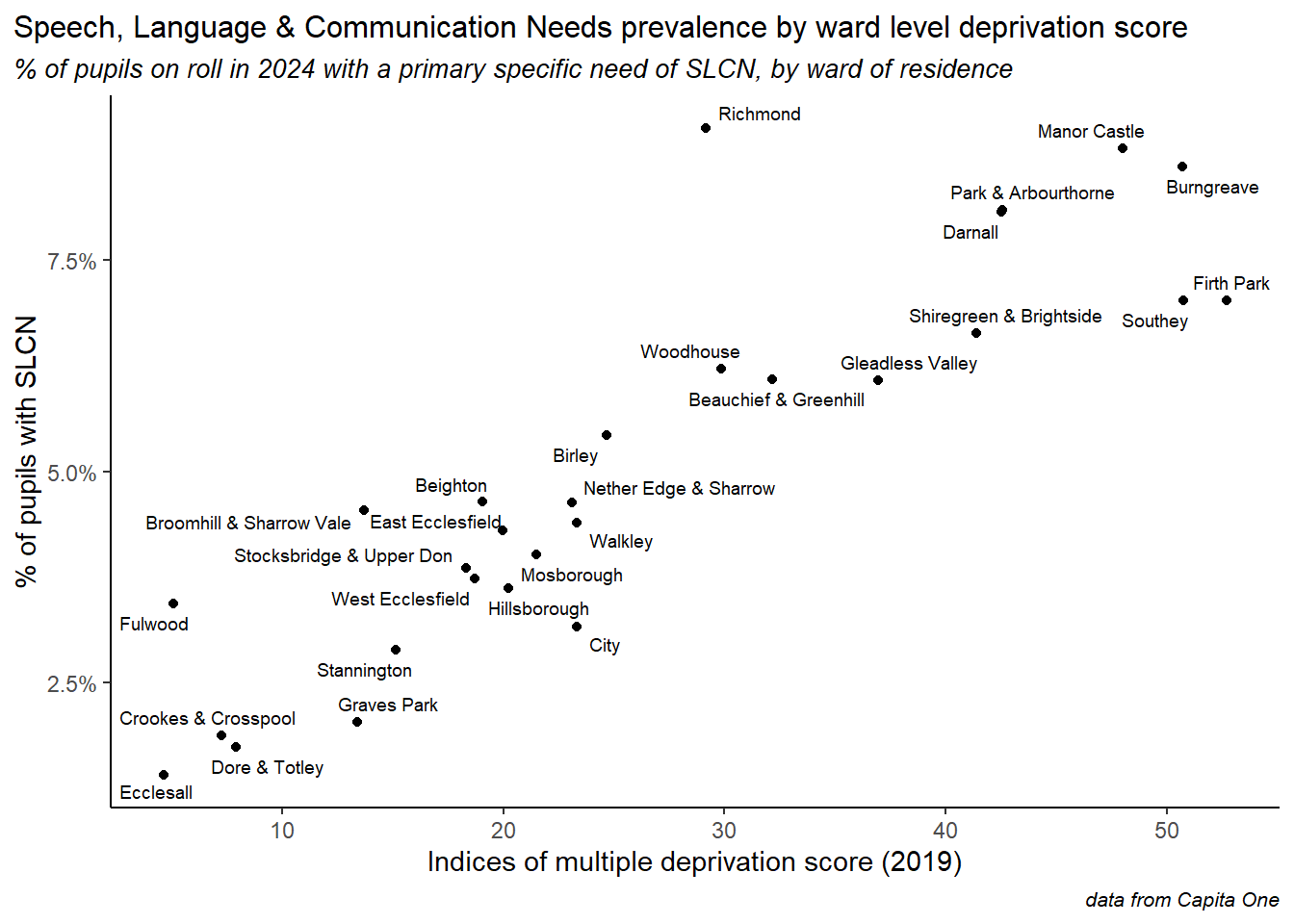
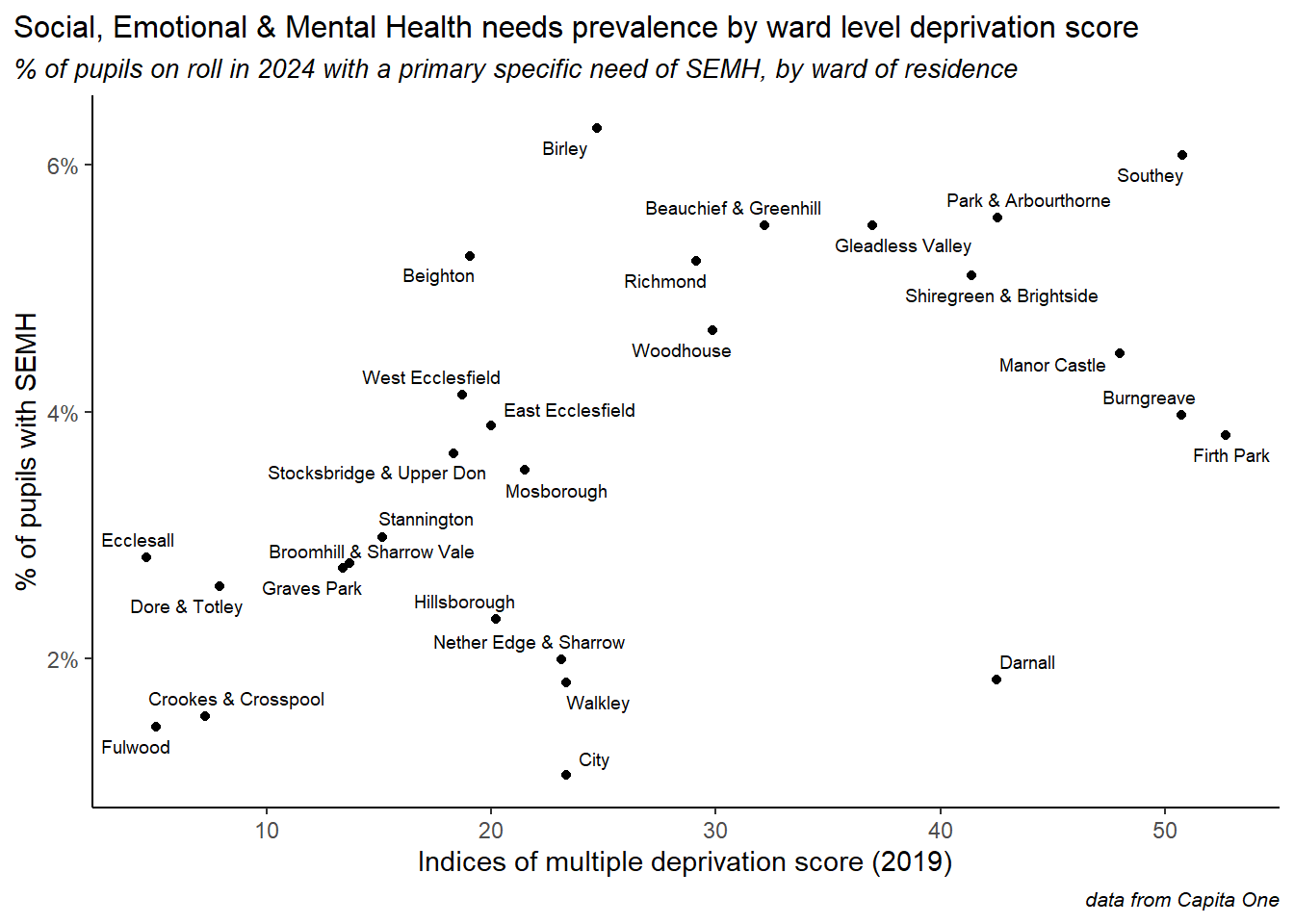
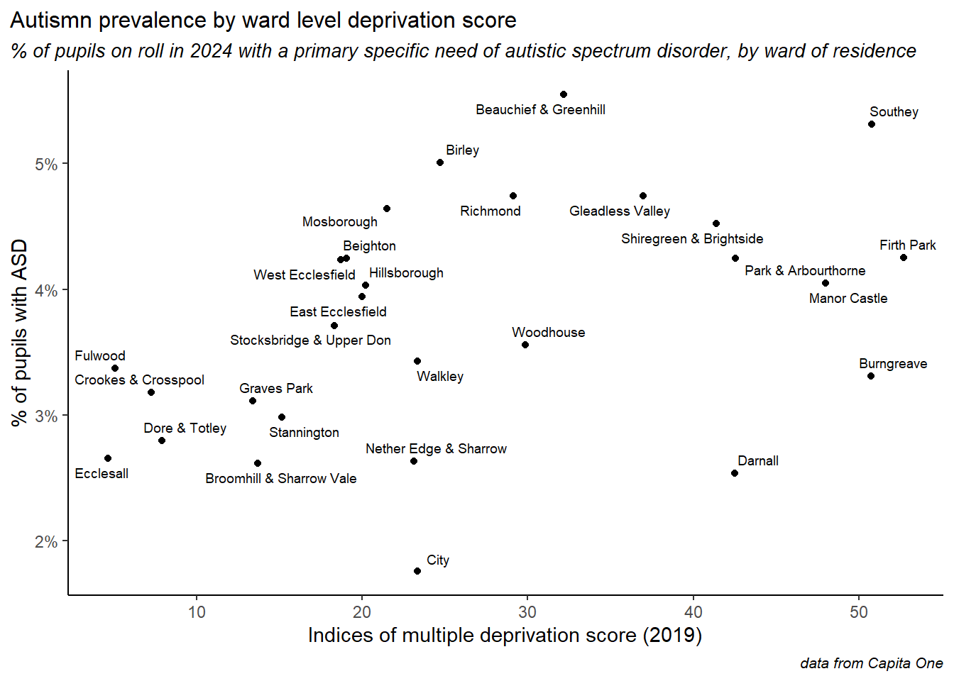
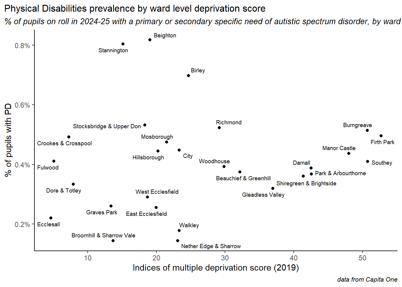
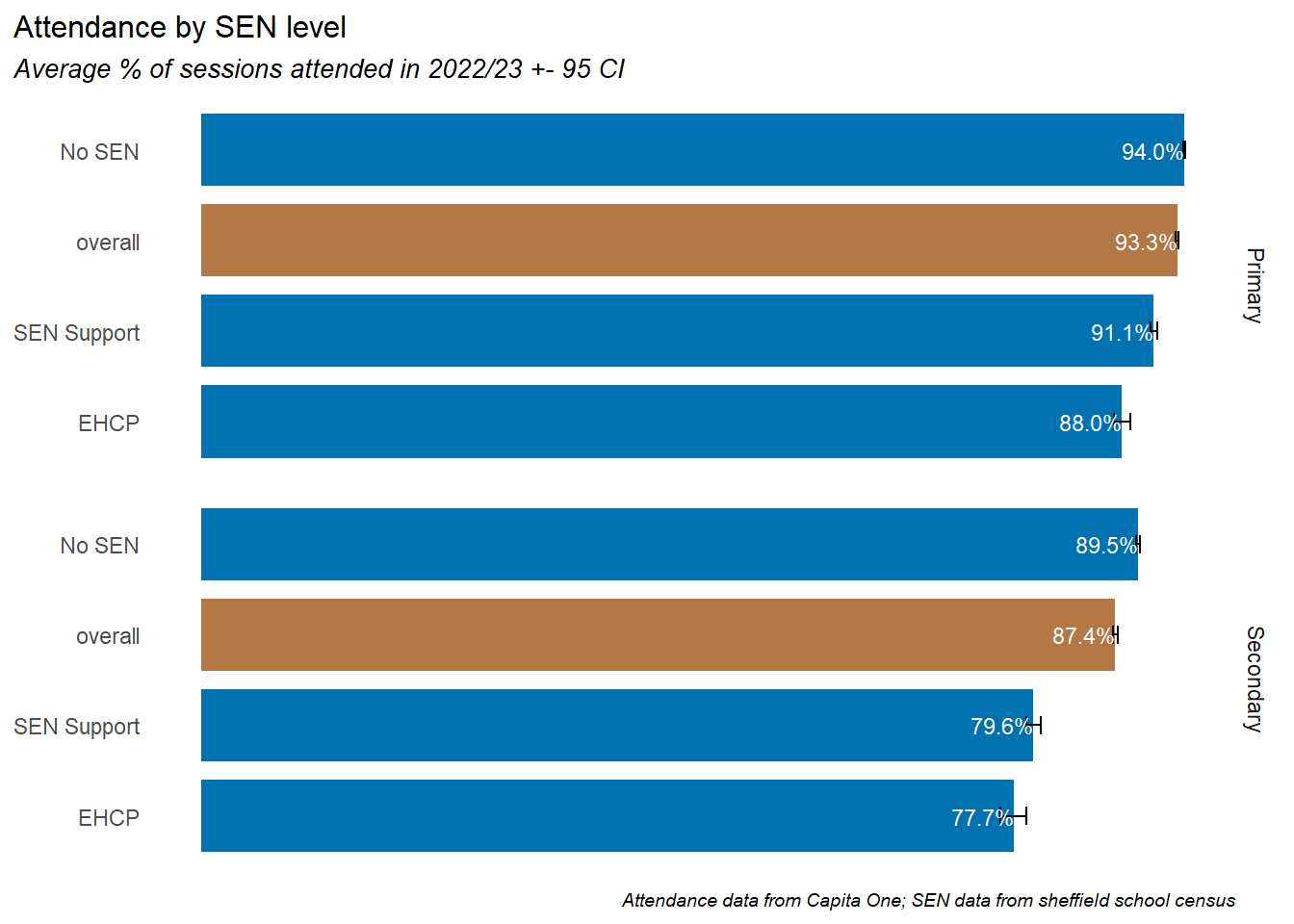
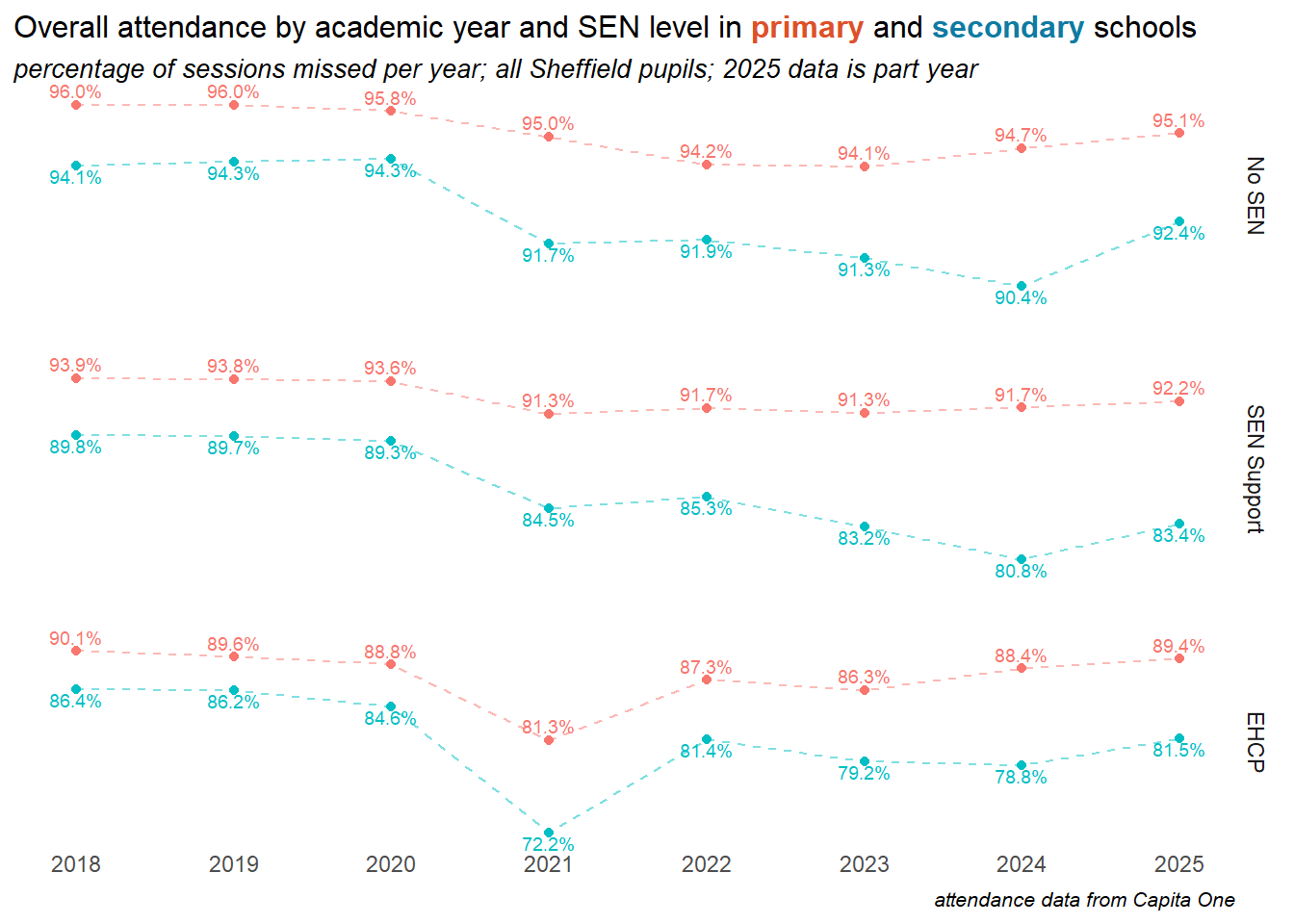
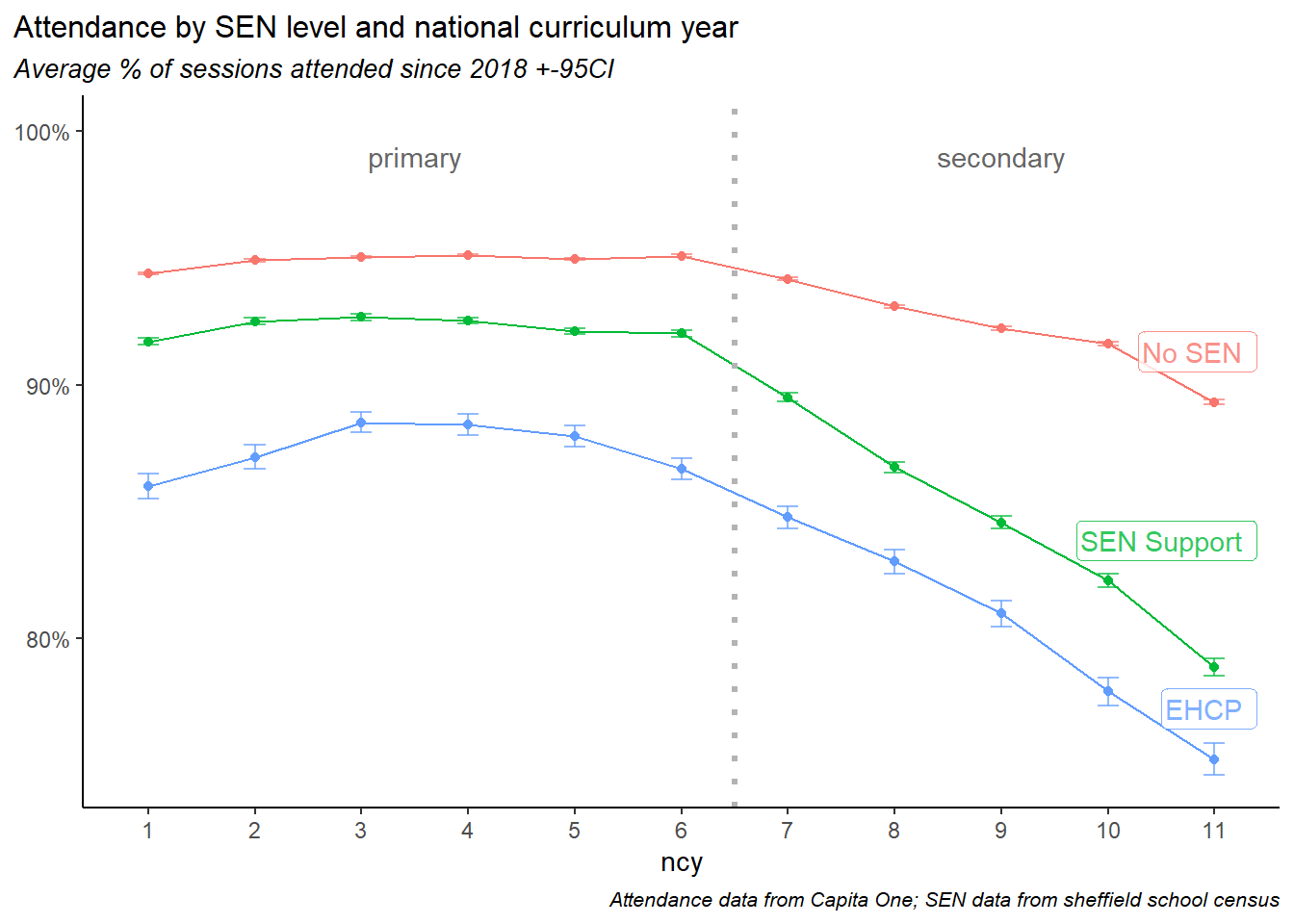
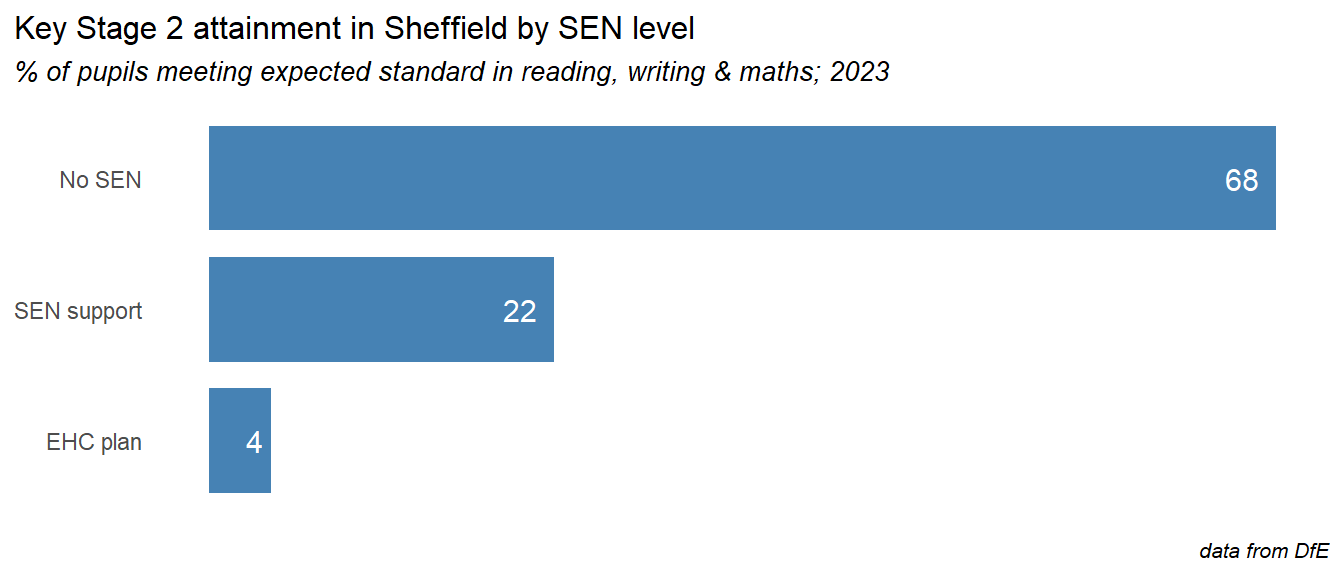
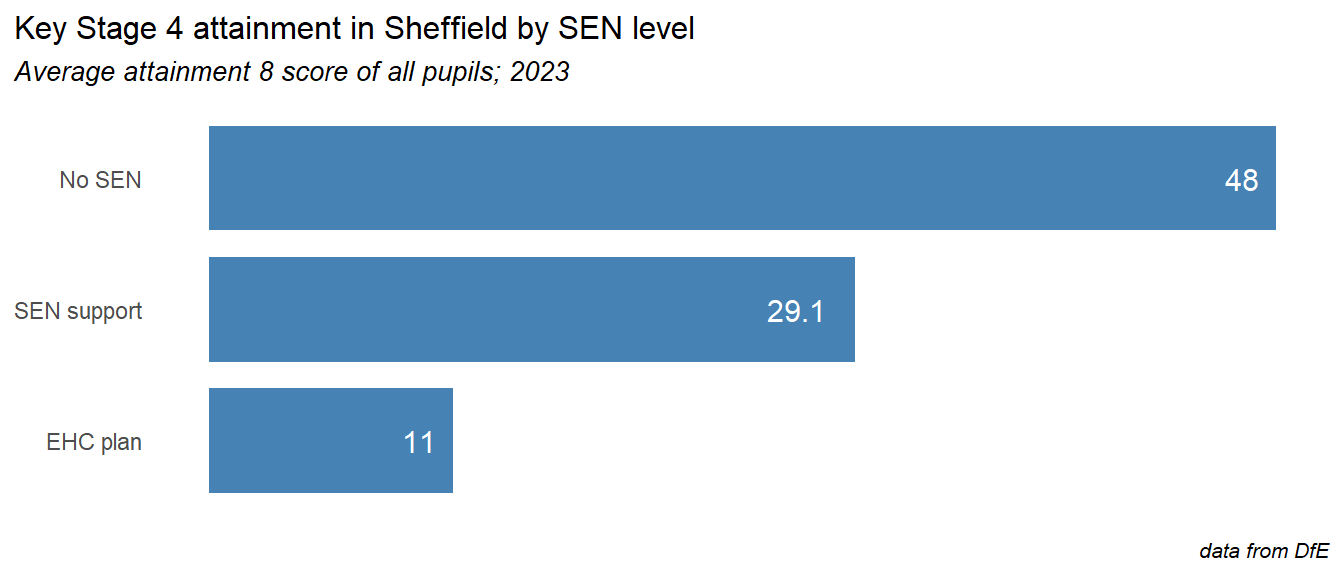
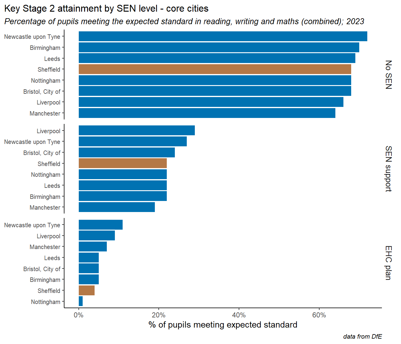
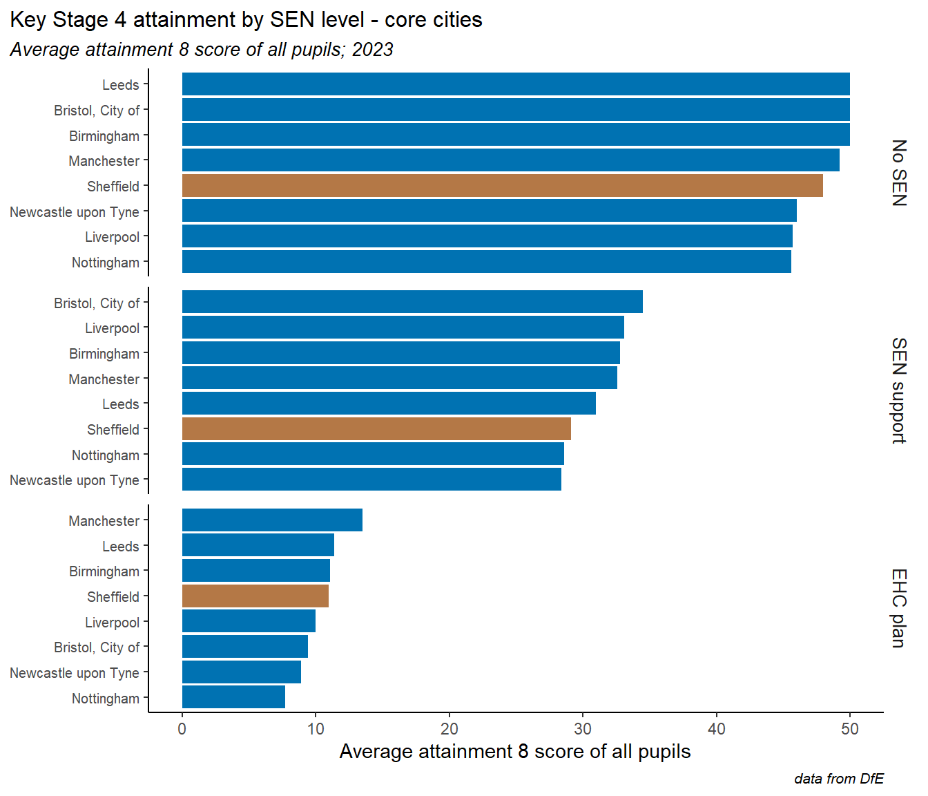
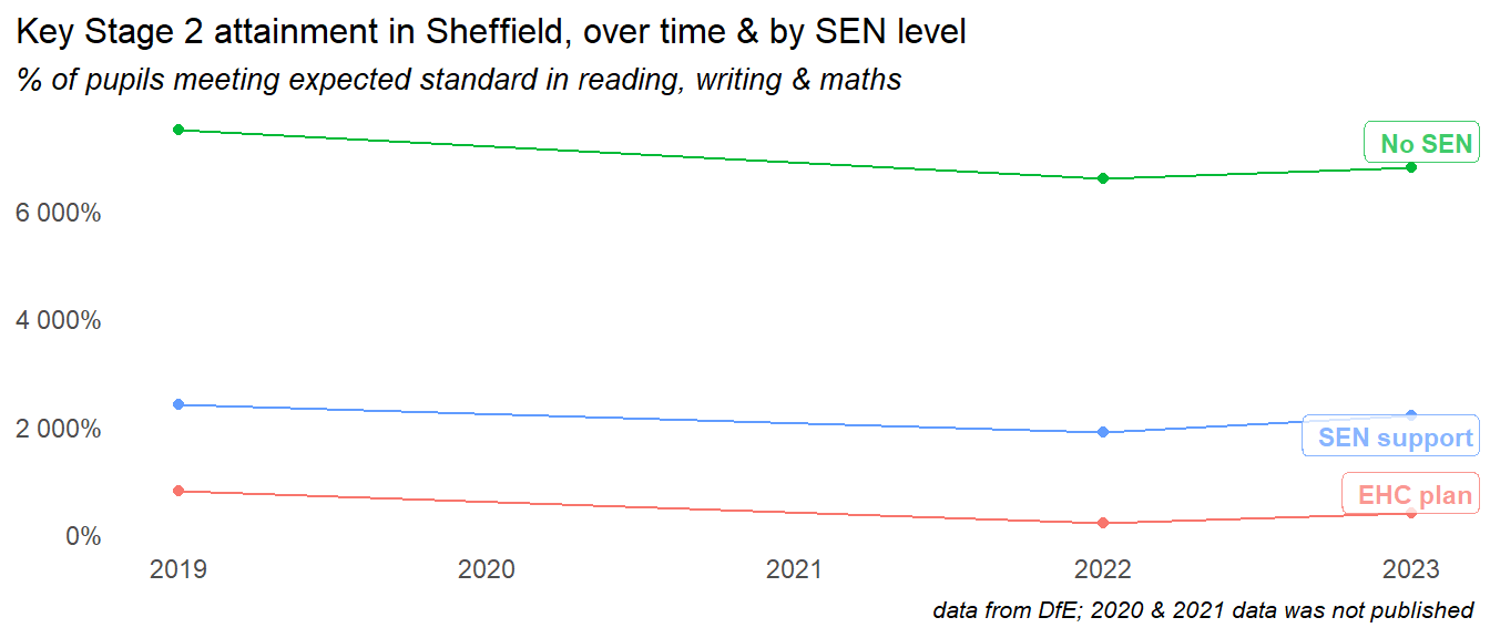
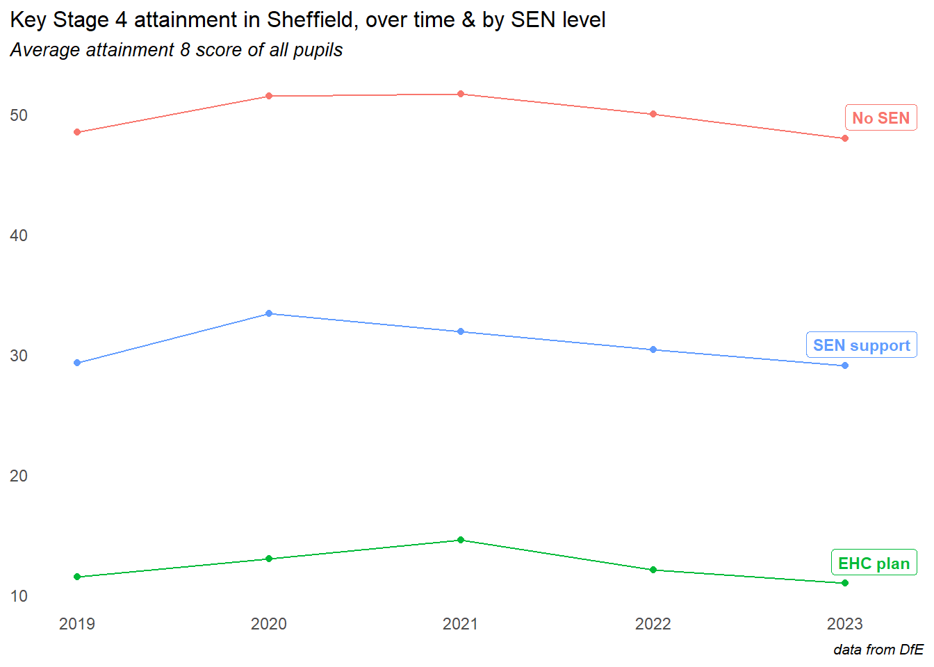
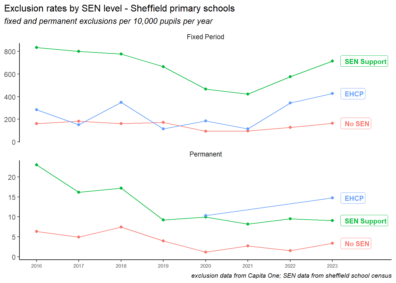
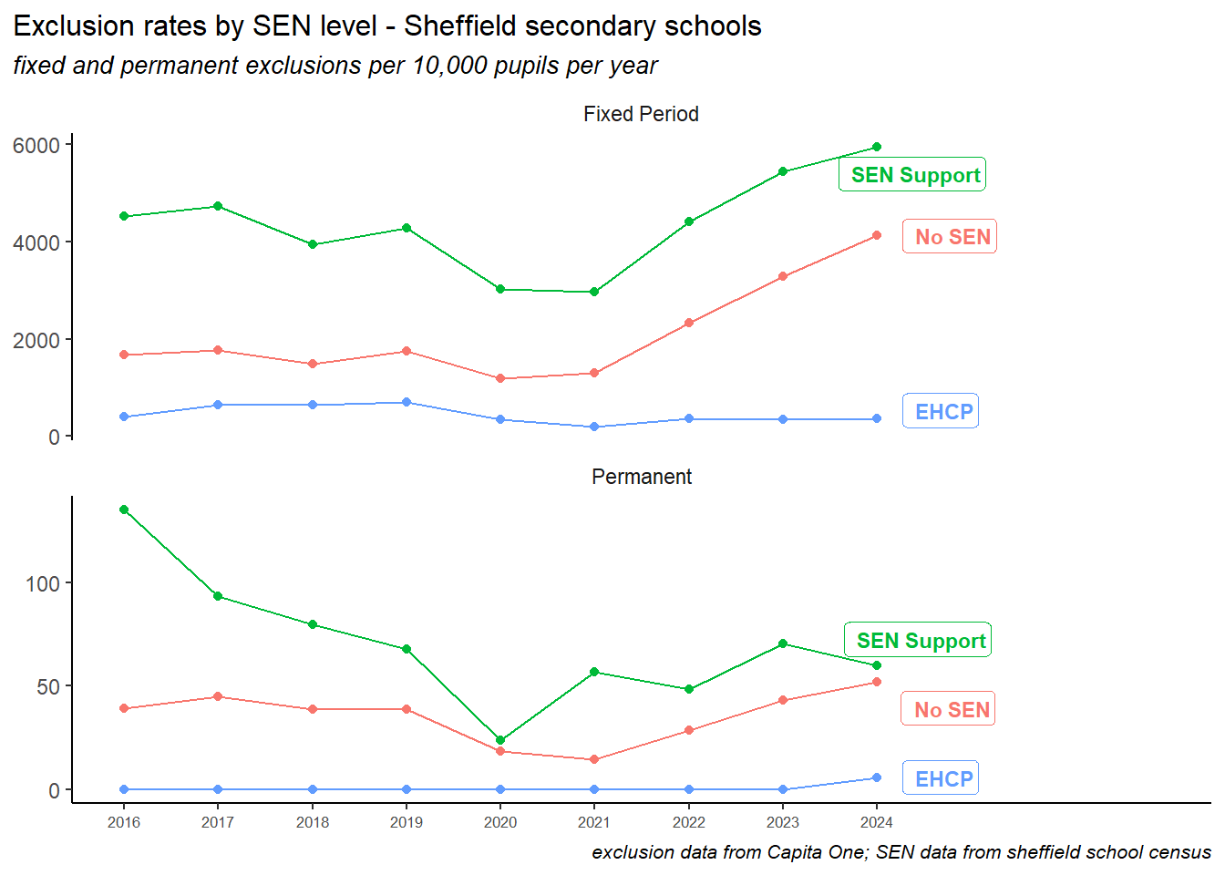
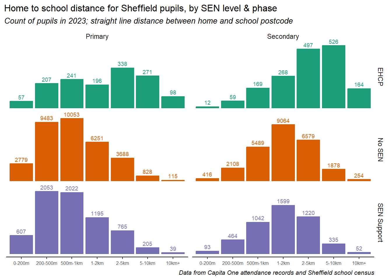
Social, Emotional & Mental Health Needs