import osimport localeimport datetimeimport pandas as pdfrom pandas.api.types import CategoricalDtypeimport numpy as npimport hl_risk as hl# https://github.com/ymrohit/ukpostcodeiofrom ukpostcodeio.client import UKPostCodeIOimport geopandas as gpdfrom plotnine import ggplot, aes, geom_line, facet_wrap, labs, theme_classic, geom_boxplot, geom_bar,geom_col,element_text, scale_y_continuous, theme, position_dodge, scale_fill_brewerimport warnings warnings.filterwarnings('ignore')# Load the homelessness case & household membership dataframeshl_case = hl.load_hl_case()hl_case_hh = hl.load_hl_case_hh()# Load the homelessness client and high level support client dataframes hl_client = hl.load_hl_client()hl_high = hl.load_hl_high()# Load the homeless households & people dataframeshl_hh = hl.load_hl_hh()hl_person = hl.load_hl_person()# Number of rows in each dataframen_hl_case = hl_case.shape[0]n_hl_case_hh = hl_case_hh.shape[0]# Earliest and last casecase_earliest_date = hl_case["application_date"].min()case_last_date = hl_case["application_date"].max()
We have data for 21,449 homelessness cases, and 32,344 records relating to the household members of homelessness cases. Our earliest homelessness case in the data is 01/04/2019 and the last is 31/03/2025.
1 Last settled postcode
What locations (last settled postcode) have the highest rates of homelessness?
Code
# Cases where last_settled_postcode is not emptyhl_case_lsp = hl_case[hl_case["last_settled_postcode"].notnull()] n_hl_case_lsp = hl_case_lsp.shape[0]pct_hl_case_lsp =round(n_hl_case_lsp/n_hl_case, 2)
Only 38% of homelessness cases have a last settled postcode value (we’ve not checked yet whether the postcode value is valid). Stephen mentioned this should be better in more recent years.
Code
# New boolean field indicating if last settled postcode is emptyhl_case["lsp_null"] = hl_case["last_settled_postcode"].isnull()# Annual count of cases where last_settled_postcode is empty and not emptyhl_case_lsp_yr = ( hl_case[["hra_case_id", "application_year", "lsp_null"]] .groupby(by=["application_year", "lsp_null"]) .size() .reset_index(name='cases'))# Reshape the tablehl_case_lsp_yr = ( hl_case_lsp_yr .pivot(index="application_year", columns="lsp_null", values="cases") .reset_index() .fillna(0) .astype({True: "int", False: "int" }))# Rename the columnshl_case_lsp_yr = hl_case_lsp_yr.rename(columns = {"application_year": "year",False: "with_postcode",True: "no_postcode"})# Total number of caseshl_case_lsp_yr["total_cases"] = ( hl_case_lsp_yr["with_postcode"] + hl_case_lsp_yr["no_postcode"])# Percentage of cases with a postcode hl_case_lsp_yr["pct_with_postcode"] = (round((hl_case_lsp_yr["with_postcode"] / hl_case_lsp_yr["total_cases"]), 2)*100)hl_case_lsp_yr = hl_case_lsp_yr.astype({"pct_with_postcode": "int"})hl_case_lsp_yr = hl_case_lsp_yr.astype({"pct_with_postcode": "str"})hl_case_lsp_yr["pct_with_postcode"] = hl_case_lsp_yr["pct_with_postcode"] +"%"( hl_case_lsp_yr[["year", "pct_with_postcode"]] .style .hide(axis ="index") .set_properties(subset = ["pct_with_postcode"], **{"text-align": "right"}))
Homelessness cases with last settled postcode
year
pct_with_postcode
2019
0%
2020
0%
2021
0%
2022
31%
2023
74%
2024
87%
2025
74%
Code
# List of postcodes # postcodes = hl_case_lsp["last_settled_postcode"].unique()[:230].tolist() # for testingpostcodes = hl_case_lsp["last_settled_postcode"].unique().tolist()# Initialize the client with default settingspostcode_client = UKPostCodeIO()# Initialize the client with custom timeout and retriespostcode_client = UKPostCodeIO(timeout=10, max_retries=5)# postcodes.io has a maximum of 100 postcode bulk lookups at a time# Loop through 100 postcodes at a timen_bulk_max =100n_postcodes =len(postcodes)bulk_loops = n_postcodes // n_bulk_maxbulk_mod = n_postcodes % n_bulk_maxif bulk_mod >0: bulk_loops +=1else: bulk_mod = n_bulk_max# Bulk lookup postcodesfor i inrange(bulk_loops): j = i +1 batch_start = j * n_bulk_max - n_bulk_max if j < bulk_loops: batch_end = j * n_bulk_maxelse: batch_end = batch_start + bulk_mod postcode_batch = postcodes[batch_start:batch_end] batch_results = postcode_client.bulk_lookup_postcodes(postcode_batch)if j ==1: results = batch_resultselse: results += batch_results# Good practice to close the client session when donepostcode_client.close()# Flatten results and extract the ward results = pd.DataFrame(results)results = results.result.apply(pd.Series)results["admin_ward_code"] = results['codes'].str.get('admin_ward')results = results[["postcode","admin_district","pfa","admin_ward","admin_ward_code"]]# We searched on unique postcodes so need to rejoinhl_case_lsp = hl_case_lsp.merge( right = results, how ="left", left_on ="last_settled_postcode", right_on ="postcode")# Identify invalid postcode and postcode outside of Sheffieldadmin_district_ft = (hl_case_lsp[["admin_district", "pfa"]] .value_counts(dropna =False) .rename("cases") .reset_index() .fillna("Invalid postcode"))# Label neighbouring districts as South Yorkshire admin_district_ft.loc[ (admin_district_ft['pfa'] =="South Yorkshire") & (admin_district_ft['admin_district'] !="Sheffield"), 'admin_district'] ="South Yorkshire"# Label "other" districtsadmin_district_ft.loc[~admin_district_ft['admin_district'].isin(["Invalid postcode","Sheffield","South Yorkshire" ]),'admin_district'] ="Other"# Group and re-sumadmin_district_ft = ( admin_district_ft .groupby("admin_district") .sum("cases") .reset_index(names="admin_district"))# Change admin_district to a category data typeadmin_district_ft["admin_district"] = ( admin_district_ft["admin_district"].astype("category"))# Apply an order to our admin_district categoriesadmin_district_order = ["Sheffield", "South Yorkshire", "Other", "Invalid postcode"]admin_district = CategoricalDtype(categories=admin_district_order, ordered=True)admin_district_ft["admin_district"] = ( admin_district_ft["admin_district"] .cat.reorder_categories(admin_district_order, ordered=True))admin_district_ft = admin_district_ft.sort_values("admin_district")( admin_district_ft .style .hide(axis ="index") .format(thousands =",") .set_properties(subset = ["cases"], **{"text-align": "right"}))
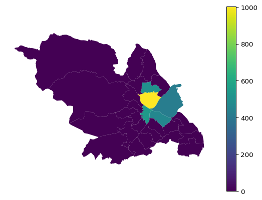
# Downloaded ward boundaries from ONS Ope Geography Portal as GeoPackage# https://geoportal.statistics.gov.uk/datasets/bd816ce7fa384745851f942786671f87_0/explore?location=59.429324%2C28.266256%2C3.58# Get Sheffield ward boundariesward_filename ="Wards_December_2024_Boundaries_UK_BFC_3254702094383695880.gpkg"wards = gpd.read_file(os.path.join(hl.get_path_local_data(), ward_filename))wards = wards[wards['LAD24NM'] =='Sheffield']# Join number of cases to ward boundarieswards = wards.merge( right = ward_cases, how ="left", left_on ="WD24NM", right_on ="admin_ward")wards[["cases"]] = wards[["cases"]].fillna(value=0)wards = wards.astype({"cases": "int"})ax = wards.plot(column='cases', legend=True)ax.set_axis_off()
Homelessness cases by ward
Is there a better geography to analyse by than Wards? TODO: Stephen has suggested the (100) neighbourhoods as an alternative set of boundaries to Wards. Housing Market Areas is another suggestion. TODO: Nicola has suggested MSOAs. This can link with census data. As a smaller area it will enabled a more in depth look at say the top 5 Wards. Plus, it may highlight some pockets that are masked by wider areas e.g. Wynn Gardens. TODO: Compare top 5 Wards with “all other Wards” . TODO: Stephen has suggested adding “last settled accommodation type” to this exploratory analysis of last settled postcode.
2 Household type
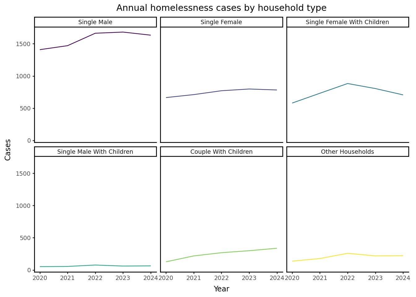
2.1 Annual
We don’t have a complete year of data for 2019 or 2025.
Code
# Number of annual cases by household typehh_type_yr = ( hl_case.loc[ (hl_case["application_year"] >2019) & (hl_case["application_year"] <2025), ["application_year", "household_type"] ] .value_counts(dropna =False) .rename("cases") .reset_index())# Title for each facetdef titled(strip_title):return" ".join(s.title() if s !="and"else s for s in strip_title.split("_"))# Facet plot( ggplot( hh_type_yr, aes(x="application_year", y="cases", colour="household_type") )+ geom_line(size=.5, show_legend=False)+ facet_wrap("household_type", labeller=titled)+ labs( x="Year", y="Cases", colour="Household type", title="Annual homelessness cases by household type" )+ theme_classic(base_size=9))
2.2 Seasonal
TODO
3 Demographic Profiling of Settled Home Loss Cases
Exploratory analysis building a profile of demographic, geographic and support need information for households presenting for specific Settled Home Loss Reasons.
3.1 Settled Home Loss Reason
What are the different settled homeloss reasons?
Code
# Frequency table for the Settled Home Loss Reason column homeloss_reason_ft = (hl_case["settled_home_loss_reason"] .value_counts(dropna =True) #missing records will be dropped or might want to keep as "Unknown" .rename("cases") .reset_index())# Format the table display( homeloss_reason_ft.style .hide(axis ="index") .format(thousands =",") .set_properties(subset = ["settled_home_loss_reason"], **{"text-align": "left"}) .set_properties(subset = ["cases"], **{"text-align": "right"}))
Frequency of Settled Home Loss Reason
settled_home_loss_reason
cases
Family no longer willing or able to accommodate
4,664
Domestic abuse - victim
2,980
End of private rented tenancy - assured shorthold tenancy
2,423
Required to leave accommodation provided by Home Office as asylum support
1,541
Friends no longer willing or able to accommodate
1,259
Domestic abuse
1,254
Relationship with partner ended (non-violent breakdown)
1,137
Other
1,031
Non-racially motivated / other motivated violence or harassment
968
Eviction from supported housing
912
Departure from institution: Custody
736
End of social rented tenancy
564
End of private rented tenancy - not assured shorthold tenancy
407
Domestic abuse - alleged perpetrator excluded from property
187
Left institution with no accommodation available
177
Fire or flood / other emergency
158
Home no longer suitable due to disability / ill health
136
Property disrepair
134
Not known due to last settled accommodation Not known
97
Racially motivated violence or harassment
92
Voluntarily left accommodation to relocate
74
Mortgage repossession or sale of owner occupier property
73
Departure from institution: Hospital (psychiatric)
44
Departure from institution: Hospital (general)
44
Left HM Forces
9
Loss of tied accommodation
8
Departure from institution: Looked After Child Placement
8
Unsuccessful placement or exclusion from resettlement scheme/sponsorship
5
3.2 Family or Friends no longer willing or able to accommodate
Focusing on two specific reasons of settled home loss:
Family no longer willing or able to accommodate.
Friends no longer willing or able to accommodate.
Code
# Define categories of interesthomeloss_reasons_fandf_categories_of_interest = ["Family no longer willing or able to accommodate", "Friends no longer willing or able to accommodate"]# Filter the data for these 2 specific reasonshomeloss_reason_fandf_filtered = hl_case[hl_case["settled_home_loss_reason"].isin(homeloss_reasons_fandf_categories_of_interest)]homeloss_reason_fandf_filtered_ft = (homeloss_reason_fandf_filtered ["settled_home_loss_reason"] .value_counts(dropna =False) .rename("cases") .reset_index())# Format the table display( homeloss_reason_fandf_filtered_ft.style .hide(axis ="index") .format(thousands =",") .set_properties(subset = ["settled_home_loss_reason"], **{"text-align": "left"}) .set_properties(subset = ["cases"], **{"text-align": "right"}))
settled_home_loss_reason
cases
Family no longer willing or able to accommodate
4,664
Friends no longer willing or able to accommodate
1,259
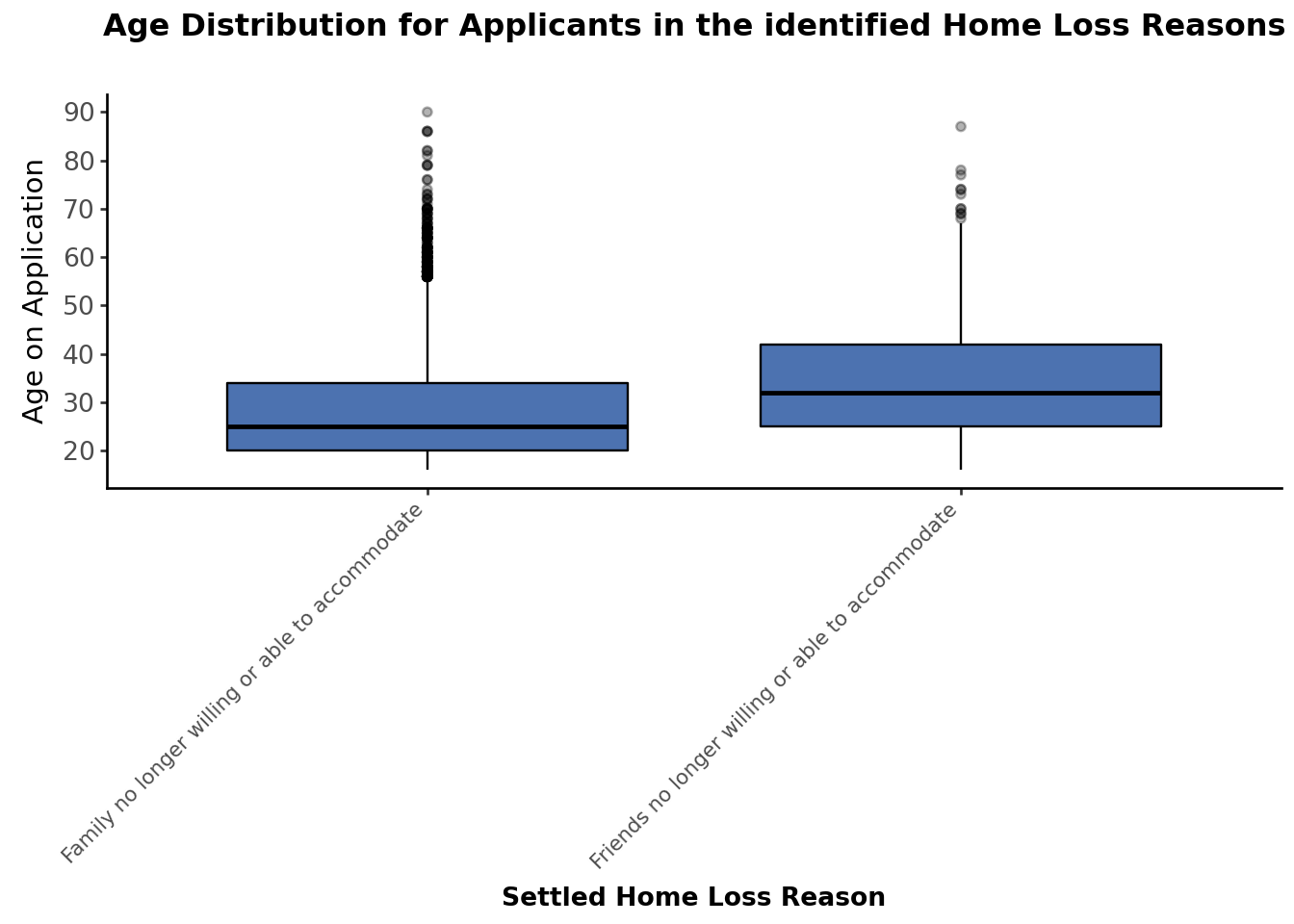
3.2.1 Breakdown by Age
Analysis of Settled Home Loss Reasons (Family or Friends no longer willing or able to accommodate) by applicant’s age at the time of application.
Code
# Age Distribution for Applicants in the identified Home Loss Reasons categories of interesthomeloss_reason_fandf_filtered["age_on_application"].describe()#Compare Age accross identified Home Loss Reasons categories of interest (Family or Friends no longer willing or able to accommodate) using a boxplot( ggplot(homeloss_reason_fandf_filtered, aes(x="settled_home_loss_reason", y="age_on_application"))+ geom_boxplot(fill="#4C72B0", color="black", outlier_alpha=0.3)+ theme_classic()+ labs( title="Age Distribution for Applicants in the identified Home Loss Reasons", x="Settled Home Loss Reason", y="Age on Application" )+ scale_y_continuous(breaks=range(0, 101, 10))+ theme( axis_text_x=element_text(rotation=45, ha="right", size=8), axis_text_y=element_text(size=10, margin={"r": 15}), axis_title_x=element_text(size=10, weight="bold"), plot_title=element_text(size=12, weight="bold", ha="center", margin={"b": 20}),#plot_margin={"t": 10, "r": 10, "b": 40, "l": 40} ))
3.2.2 Breakdown by Age Group
Analysis of Settled Home Loss Reasons (Family or Friends no longer willing or able to accommodate) by applicant’s age group.
Code
# Age Group Distribution for Applicants in the identified Home Loss Reasons categories of interest#Create Age Groups#Age groups definedage_bins = [0,25,35,45,55,65,75,85,100]age_labels = ["24 and under", "25-34", "35-44", "45-54", "55-64", "65-74", "75-84", "85 and over"] #New Column for Age Grouphomeloss_reason_fandf_filtered["age_group"] = pd.cut(homeloss_reason_fandf_filtered["age_on_application"], bins=age_bins, labels=age_labels, right=False) #Age Group distributionhomeloss_reason_fandf_filtered["age_group"].value_counts()# Create table by Age groups and settled_home_loss_reasonhomeloss_reason_fandf_age_group_ft = ( homeloss_reason_fandf_filtered.groupby( ["settled_home_loss_reason", "age_group"]) .size() .unstack(fill_value=0) .reset_index())# Format the table display( homeloss_reason_fandf_age_group_ft.style .hide(axis ="index") .format(thousands =",") .set_properties(**{"text-align": "center"}) .set_properties(subset = ["settled_home_loss_reason"], **{"text-align": "left"}))
settled_home_loss_reason
24 and under
25-34
35-44
45-54
55-64
65-74
75-84
85 and over
Family no longer willing or able to accommodate
2,209
1,343
596
300
161
43
8
4
Friends no longer willing or able to accommodate
291
413
289
160
87
16
2
1
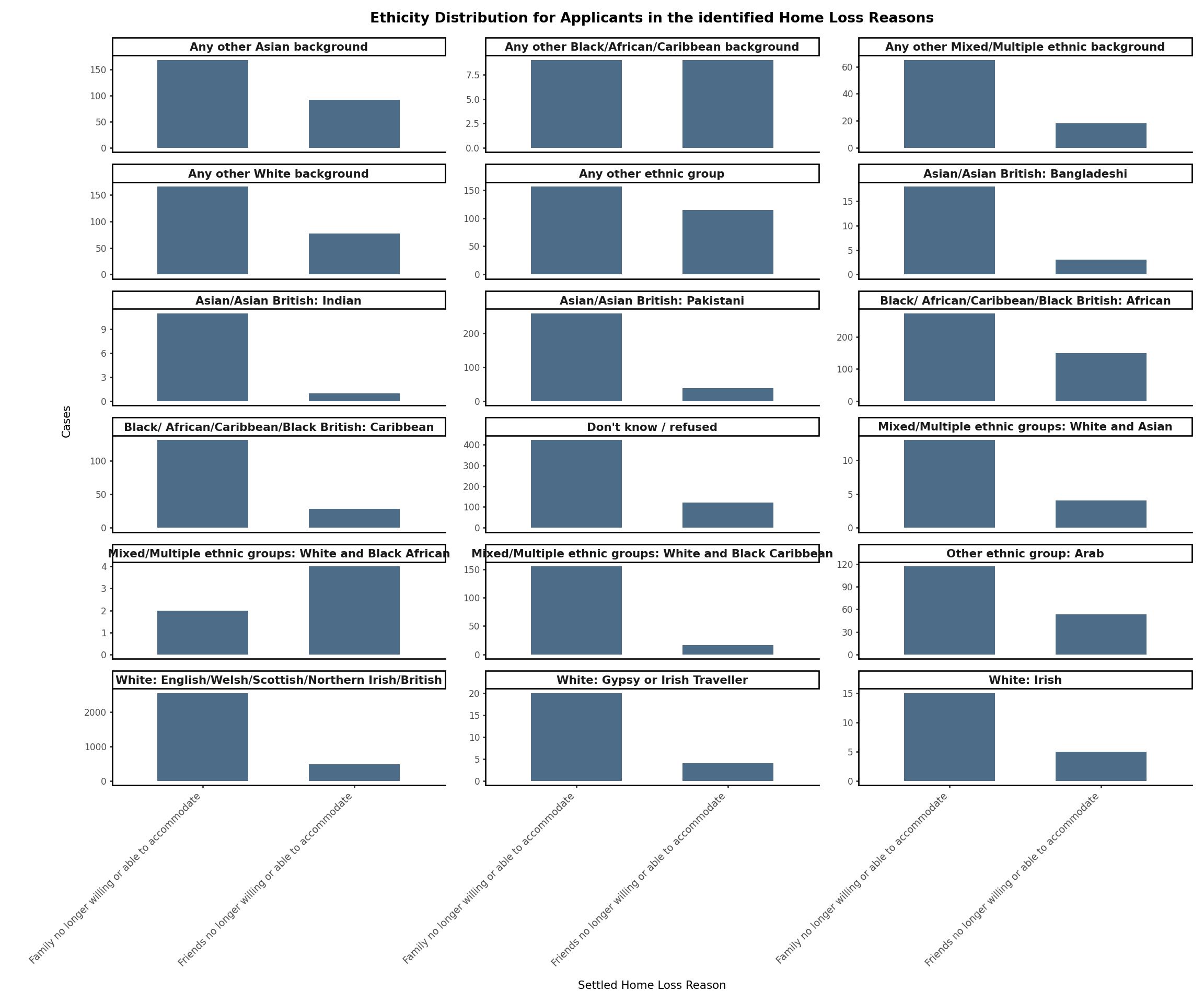
3.2.3 Breakdown by Ethnicity
Analysis of Settled Home Loss Reasons (Family or Friends no longer willing or able to accommodate) by applicant’s ethnicity.
Code
# Ethnicity Distribution for Applicants in the identified Home Loss Reasons categories of interesthomeloss_reason_fandf_filtered["ethnicity"].value_counts()# Create table by Ethnicity and settled_home_loss_reasonhomeloss_reason_fandf_ethnicity_ft = (homeloss_reason_fandf_filtered .groupby( ["ethnicity","settled_home_loss_reason"]) .size() .unstack(fill_value=0) .reset_index())# Sort by Total cases in descending orderhomeloss_reason_fandf_ethnicity_ft["Total"] = homeloss_reason_fandf_ethnicity_ft.iloc[:, 1:].sum(axis=1)homeloss_reason_fandf_ethnicity_ft = homeloss_reason_fandf_ethnicity_ft.sort_values("Total", ascending=False).drop(columns="Total")# Format the table display( homeloss_reason_fandf_ethnicity_ft.style .hide(axis ="index") .format(thousands =",") .set_properties(subset = ["ethnicity"], **{"text-align": "left"}) .set_properties(subset = homeloss_reason_fandf_ethnicity_ft.columns[1:], **{"text-align": "right"}))
Mixed/Multiple ethnic groups: White and Black Caribbean
155
16
Other ethnic group: Arab
117
53
Black/ African/Caribbean/Black British: Caribbean
131
28
Any other Mixed/Multiple ethnic background
65
18
White: Gypsy or Irish Traveller
20
4
Asian/Asian British: Bangladeshi
18
3
White: Irish
15
5
Any other Black/African/Caribbean background
9
9
Mixed/Multiple ethnic groups: White and Asian
13
4
Asian/Asian British: Indian
11
1
Mixed/Multiple ethnic groups: White and Black African
2
4
Code
#Compare Ethnicity accross identified Home Loss Reasons categories of interest (Family or Friends no longer willing or able to accommodate)# Melt to long format homeloss_reason_fandf_ethnicity_long = homeloss_reason_fandf_ethnicity_ft.melt(id_vars="ethnicity", var_name="settled_home_loss_reason", value_name="cases")# Create a Facet plot( ggplot(homeloss_reason_fandf_ethnicity_long, aes(x="settled_home_loss_reason", y="cases"))+ geom_col(fill="#4c6c88", width=0.6)+ facet_wrap("~ethnicity", labeller="label_value", scales="free_y", ncol=3)+ theme_classic(base_size=8)+ labs( title="Ethicity Distribution for Applicants in the identified Home Loss Reasons", x="Settled Home Loss Reason", y="Cases" )+ theme( axis_text_x=element_text(rotation=45, ha="right", size=7), figure_size=(12, 10), strip_text=element_text(weight="bold", size=8), plot_title=element_text(size=10, weight="bold") ))
3.3 End of private rented tenancy
Focusing on two specific reasons of settled home loss:
End of private rented tenancy - assured shorthold tenancy.
End of private rented tenancy - not assured shorthold tenancy.
Code
# Define categories of interesthomeloss_reasons_ept_categories_of_interest = ["End of private rented tenancy - assured shorthold tenancy", "End of private rented tenancy - not assured shorthold tenancy"]# Filter the data for these 2 specific reasonshomeloss_reason_ept_filtered = hl_case[hl_case["settled_home_loss_reason"].isin(homeloss_reasons_ept_categories_of_interest)]homeloss_reason_ept_filtered_ft = (homeloss_reason_ept_filtered ["settled_home_loss_reason"] .value_counts(dropna =False) .rename("cases") .reset_index())# Format the table display( homeloss_reason_ept_filtered_ft.style .hide(axis ="index") .format(thousands =",") .set_properties(subset = ["settled_home_loss_reason"], **{"text-align": "left"}) .set_properties(subset = ["cases"], **{"text-align": "right"}))
settled_home_loss_reason
cases
End of private rented tenancy - assured shorthold tenancy
2,423
End of private rented tenancy - not assured shorthold tenancy
407
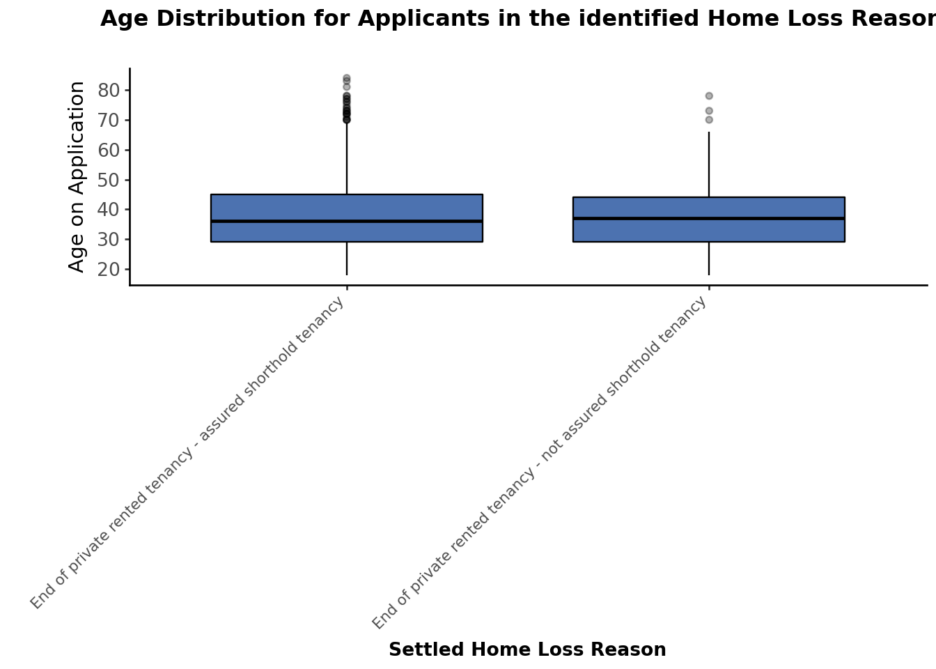
3.3.1 Breakdown by Age
Analysis of Settled Home Loss Reasons (End of private rented tenancy) by applicant’s age at the time of application.
Code
# Age Distribution for Applicants in the identified Home Loss Reasons categories of interesthomeloss_reason_ept_filtered["age_on_application"].describe()#Compare Age accross identified Home Loss Reasons categories of interest (End of private rented tenancy) using a boxplot( ggplot(homeloss_reason_ept_filtered, aes(x="settled_home_loss_reason", y="age_on_application"))+ geom_boxplot(fill="#4C72B0", color="black", outlier_alpha=0.3)+ theme_classic()+ labs( title="Age Distribution for Applicants in the identified Home Loss Reasons", x="Settled Home Loss Reason", y="Age on Application" )+ scale_y_continuous(breaks=range(0, 101, 10))+ theme( axis_text_x=element_text(rotation=45, ha="right", size=8), axis_text_y=element_text(size=10, margin={"r": 15}), axis_title_x=element_text(size=10, weight="bold"), plot_title=element_text(size=12, weight="bold", ha="center", margin={"b": 20}),#plot_margin={"t": 10, "r": 10, "b": 40, "l": 40} ))
3.3.2 Breakdown by Age Group
Analysis of Settled Home Loss Reasons (End of private rented tenancy) by applicant’s age group
Code
# Age Group Distribution for Applicants in the identified Home Loss Reasons categories of interest#Create Age Groups#Age groups definedage_bins = [0,25,35,45,55,65,75,85,100]age_labels = ["24 and under", "25-34", "35-44", "45-54", "55-64", "65-74", "75-84", "85 and over"] #New Column for Age Grouphomeloss_reason_ept_filtered["age_group"] = pd.cut(homeloss_reason_ept_filtered["age_on_application"], bins=age_bins, labels=age_labels, right=False) #Age Group distributionhomeloss_reason_ept_filtered["age_group"].value_counts()# Create table by Age groups and settled_home_loss_reasonhomeloss_reason_ept_age_group_ft = ( homeloss_reason_ept_filtered.groupby( ["settled_home_loss_reason", "age_group"]) .size() .unstack(fill_value=0) .reset_index())# Format the table display( homeloss_reason_ept_age_group_ft.style .hide(axis ="index") .format(thousands =",") .set_properties(**{"text-align": "center"}) .set_properties(subset = ["settled_home_loss_reason"], **{"text-align": "left"}))
settled_home_loss_reason
24 and under
25-34
35-44
45-54
55-64
65-74
75-84
85 and over
End of private rented tenancy - assured shorthold tenancy
242
818
726
401
187
39
10
0
End of private rented tenancy - not assured shorthold tenancy
52
124
134
64
28
4
1
0
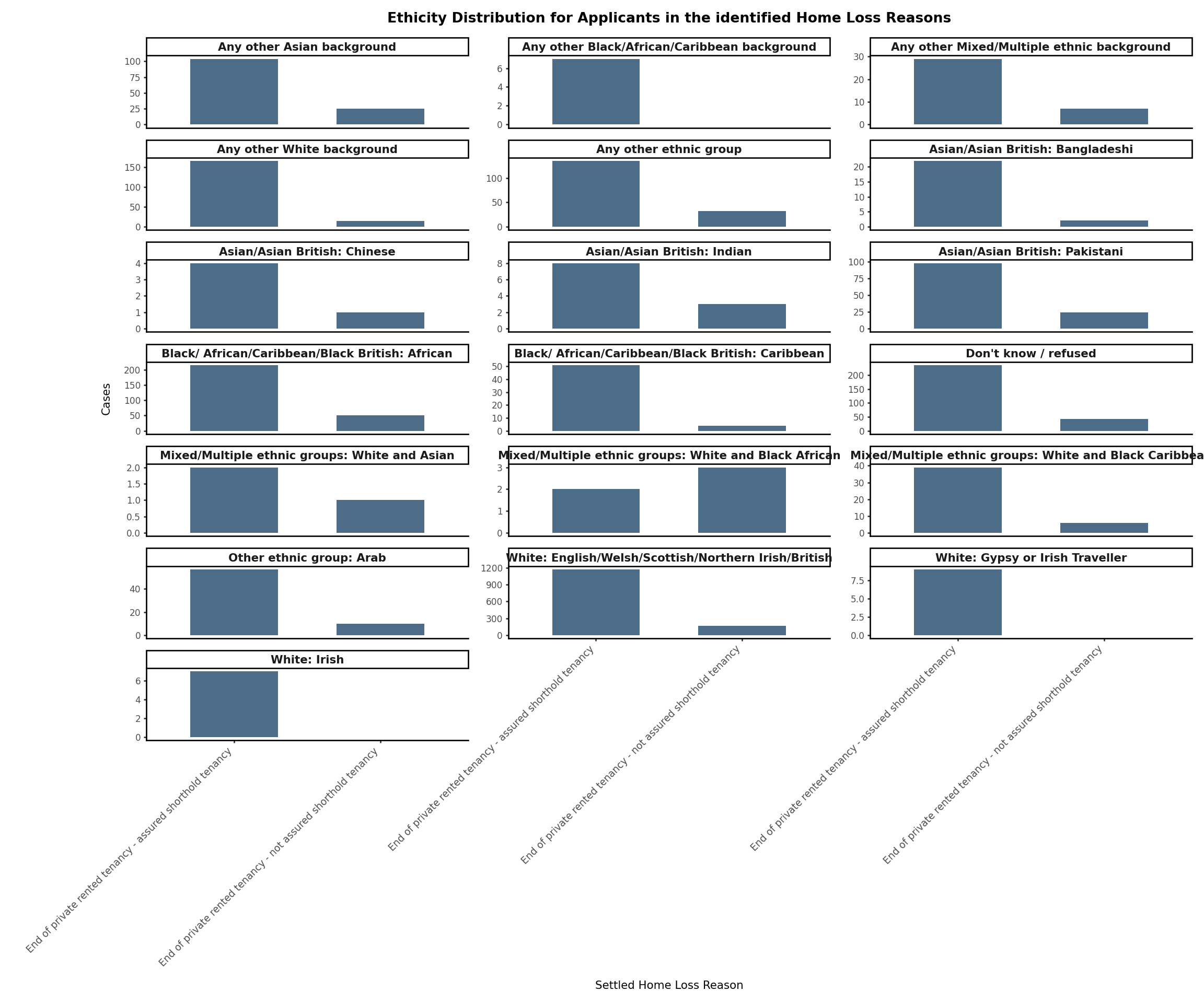
3.3.3 Breakdown by Ethnicity
Analysis of Settled Home Loss Reasons (End of private rented tenancy) by applicant’s ethnicity.
Code
# Ethnicity Distribution for Applicants in the identified Home Loss Reasons categories of interesthomeloss_reason_ept_filtered["ethnicity"].value_counts()# Create table by Ethnicity and settled_home_loss_reasonhomeloss_reason_ept_ethnicity_ft = (homeloss_reason_ept_filtered .groupby( ["ethnicity","settled_home_loss_reason"]) .size() .unstack(fill_value=0) .reset_index())# Sort by Total cases in descending orderhomeloss_reason_ept_ethnicity_ft["Total"] = homeloss_reason_ept_ethnicity_ft.iloc[:, 1:].sum(axis=1)homeloss_reason_ept_ethnicity_ft = homeloss_reason_ept_ethnicity_ft.sort_values("Total", ascending=False).drop(columns="Total")# Format the table display( homeloss_reason_ept_ethnicity_ft.style .hide(axis ="index") .format(thousands =",") .set_properties(subset = ["ethnicity"], **{"text-align": "left"}) .set_properties(subset = homeloss_reason_ept_ethnicity_ft.columns[1:], **{"text-align": "right"}))
ethnicity
End of private rented tenancy - assured shorthold tenancy
End of private rented tenancy - not assured shorthold tenancy
Mixed/Multiple ethnic groups: White and Black Caribbean
39
6
Any other Mixed/Multiple ethnic background
29
7
Asian/Asian British: Bangladeshi
22
2
Asian/Asian British: Indian
8
3
White: Gypsy or Irish Traveller
9
0
Any other Black/African/Caribbean background
7
0
White: Irish
7
0
Asian/Asian British: Chinese
4
1
Mixed/Multiple ethnic groups: White and Black African
2
3
Mixed/Multiple ethnic groups: White and Asian
2
1
Code
#Compare Ethnicity accross identified Home Loss Reasons categories of interest (Family or Friends no longer willing or able to accommodate)# Melt to long format homeloss_reason_ept_ethnicity_long = homeloss_reason_ept_ethnicity_ft.melt(id_vars="ethnicity", var_name="settled_home_loss_reason", value_name="cases")# Create a Facet plot( ggplot(homeloss_reason_ept_ethnicity_long, aes(x="settled_home_loss_reason", y="cases"))+ geom_col(fill="#4c6c88", width=0.6)+ facet_wrap("~ethnicity", labeller="label_value", scales="free_y", ncol=3)+ theme_classic(base_size=8)+ labs( title="Ethicity Distribution for Applicants in the identified Home Loss Reasons", x="Settled Home Loss Reason", y="Cases" )+ theme( axis_text_x=element_text(rotation=45, ha="right", size=7), figure_size=(12, 10), strip_text=element_text(weight="bold", size=8), plot_title=element_text(size=10, weight="bold") ))
3.3.4 Geographic Profile
TODO
Source Code
---title: "Exploratory analysis"subtitle: "Homelessness Risk"author: "Laurie Platt & Olumide Ogunyanwo"date: last-modifieddate-format: "[Last updated ] DD MMMM, YYYY"format: html: code-tools: true code-fold: true toc: true toc-location: left toc-depth: 5 toc-expand: 1 number-sections: true fig-cap-location: top code-links: - text: dev.azure.com/.../homeless-risk icon: git href: https://dev.azure.com/SheffieldCityCouncil/DataScience/_git/homeless-riskexecute: warning: false message: falseinclude-in-header: - text: | <style> .table { width: auto; } </style>---```{python}#| label: setup#| context: setupimport osimport localeimport datetimeimport pandas as pdfrom pandas.api.types import CategoricalDtypeimport numpy as npimport hl_risk as hl# https://github.com/ymrohit/ukpostcodeiofrom ukpostcodeio.client import UKPostCodeIOimport geopandas as gpdfrom plotnine import ggplot, aes, geom_line, facet_wrap, labs, theme_classic, geom_boxplot, geom_bar,geom_col,element_text, scale_y_continuous, theme, position_dodge, scale_fill_brewerimport warnings warnings.filterwarnings('ignore')# Load the homelessness case & household membership dataframeshl_case = hl.load_hl_case()hl_case_hh = hl.load_hl_case_hh()# Load the homelessness client and high level support client dataframes hl_client = hl.load_hl_client()hl_high = hl.load_hl_high()# Load the homeless households & people dataframeshl_hh = hl.load_hl_hh()hl_person = hl.load_hl_person()# Number of rows in each dataframen_hl_case = hl_case.shape[0]n_hl_case_hh = hl_case_hh.shape[0]# Earliest and last casecase_earliest_date = hl_case["application_date"].min()case_last_date = hl_case["application_date"].max()```We have data for `{python} f"{n_hl_case:,}"` homelessness cases, and `{python} f"{n_hl_case_hh:,}"` records relating to the household members of homelessness cases. Our earliest homelessness case in the data is `{python} case_earliest_date.strftime("%d/%m/%Y")` and the last is `{python} case_last_date.strftime("%d/%m/%Y")`. # Last settled postcode > What locations (last settled postcode) have the highest rates of homelessness?```{python}#| label: empty-postcodes# Cases where last_settled_postcode is not emptyhl_case_lsp = hl_case[hl_case["last_settled_postcode"].notnull()] n_hl_case_lsp = hl_case_lsp.shape[0]pct_hl_case_lsp =round(n_hl_case_lsp/n_hl_case, 2)```Only `{python} f"{pct_hl_case_lsp:.0%}"` of homelessness cases have a last settled postcode value (we've not checked yet whether the postcode value is valid). Stephen mentioned this should be better in more recent years.```{python}#| label: empty-postcodes-yr#| tbl-cap: "Homelessness cases with last settled postcode"# New boolean field indicating if last settled postcode is emptyhl_case["lsp_null"] = hl_case["last_settled_postcode"].isnull()# Annual count of cases where last_settled_postcode is empty and not emptyhl_case_lsp_yr = ( hl_case[["hra_case_id", "application_year", "lsp_null"]] .groupby(by=["application_year", "lsp_null"]) .size() .reset_index(name='cases'))# Reshape the tablehl_case_lsp_yr = ( hl_case_lsp_yr .pivot(index="application_year", columns="lsp_null", values="cases") .reset_index() .fillna(0) .astype({True: "int", False: "int" }))# Rename the columnshl_case_lsp_yr = hl_case_lsp_yr.rename(columns = {"application_year": "year",False: "with_postcode",True: "no_postcode"})# Total number of caseshl_case_lsp_yr["total_cases"] = ( hl_case_lsp_yr["with_postcode"] + hl_case_lsp_yr["no_postcode"])# Percentage of cases with a postcode hl_case_lsp_yr["pct_with_postcode"] = (round((hl_case_lsp_yr["with_postcode"] / hl_case_lsp_yr["total_cases"]), 2)*100)hl_case_lsp_yr = hl_case_lsp_yr.astype({"pct_with_postcode": "int"})hl_case_lsp_yr = hl_case_lsp_yr.astype({"pct_with_postcode": "str"})hl_case_lsp_yr["pct_with_postcode"] = hl_case_lsp_yr["pct_with_postcode"] +"%"( hl_case_lsp_yr[["year", "pct_with_postcode"]] .style .hide(axis ="index") .set_properties(subset = ["pct_with_postcode"], **{"text-align": "right"}))``````{python}#| label: ukpostcodeio#| tbl-cap: "Postcode locations"# List of postcodes # postcodes = hl_case_lsp["last_settled_postcode"].unique()[:230].tolist() # for testingpostcodes = hl_case_lsp["last_settled_postcode"].unique().tolist()# Initialize the client with default settingspostcode_client = UKPostCodeIO()# Initialize the client with custom timeout and retriespostcode_client = UKPostCodeIO(timeout=10, max_retries=5)# postcodes.io has a maximum of 100 postcode bulk lookups at a time# Loop through 100 postcodes at a timen_bulk_max =100n_postcodes =len(postcodes)bulk_loops = n_postcodes // n_bulk_maxbulk_mod = n_postcodes % n_bulk_maxif bulk_mod >0: bulk_loops +=1else: bulk_mod = n_bulk_max# Bulk lookup postcodesfor i inrange(bulk_loops): j = i +1 batch_start = j * n_bulk_max - n_bulk_max if j < bulk_loops: batch_end = j * n_bulk_maxelse: batch_end = batch_start + bulk_mod postcode_batch = postcodes[batch_start:batch_end] batch_results = postcode_client.bulk_lookup_postcodes(postcode_batch)if j ==1: results = batch_resultselse: results += batch_results# Good practice to close the client session when donepostcode_client.close()# Flatten results and extract the ward results = pd.DataFrame(results)results = results.result.apply(pd.Series)results["admin_ward_code"] = results['codes'].str.get('admin_ward')results = results[["postcode","admin_district","pfa","admin_ward","admin_ward_code"]]# We searched on unique postcodes so need to rejoinhl_case_lsp = hl_case_lsp.merge( right = results, how ="left", left_on ="last_settled_postcode", right_on ="postcode")# Identify invalid postcode and postcode outside of Sheffieldadmin_district_ft = (hl_case_lsp[["admin_district", "pfa"]] .value_counts(dropna =False) .rename("cases") .reset_index() .fillna("Invalid postcode"))# Label neighbouring districts as South Yorkshire admin_district_ft.loc[ (admin_district_ft['pfa'] =="South Yorkshire") & (admin_district_ft['admin_district'] !="Sheffield"), 'admin_district'] ="South Yorkshire"# Label "other" districtsadmin_district_ft.loc[~admin_district_ft['admin_district'].isin(["Invalid postcode","Sheffield","South Yorkshire" ]),'admin_district'] ="Other"# Group and re-sumadmin_district_ft = ( admin_district_ft .groupby("admin_district") .sum("cases") .reset_index(names="admin_district"))# Change admin_district to a category data typeadmin_district_ft["admin_district"] = ( admin_district_ft["admin_district"].astype("category"))# Apply an order to our admin_district categoriesadmin_district_order = ["Sheffield", "South Yorkshire", "Other", "Invalid postcode"]admin_district = CategoricalDtype(categories=admin_district_order, ordered=True)admin_district_ft["admin_district"] = ( admin_district_ft["admin_district"] .cat.reorder_categories(admin_district_order, ordered=True))admin_district_ft = admin_district_ft.sort_values("admin_district")( admin_district_ft .style .hide(axis ="index") .format(thousands =",") .set_properties(subset = ["cases"], **{"text-align": "right"}))``````{python}#| label: ward-cases#| tbl-cap: "Wards with the most homelessness cases"# Summary table of homelessness cases by wardward_cases = ( hl_case_lsp[hl_case_lsp["admin_district"] =="Sheffield"] .groupby("admin_ward") .size() .reset_index(name='cases')).sort_values("cases", ascending =False).head()( ward_cases .style .hide(axis ="index") .format(thousands =",") .set_properties(subset = ["cases"], **{"text-align": "right"}))``````{python}#| label: map-ward-cases#| fig-cap: "Homelessness cases by ward"# Downloaded ward boundaries from ONS Ope Geography Portal as GeoPackage# https://geoportal.statistics.gov.uk/datasets/bd816ce7fa384745851f942786671f87_0/explore?location=59.429324%2C28.266256%2C3.58# Get Sheffield ward boundariesward_filename ="Wards_December_2024_Boundaries_UK_BFC_3254702094383695880.gpkg"wards = gpd.read_file(os.path.join(hl.get_path_local_data(), ward_filename))wards = wards[wards['LAD24NM'] =='Sheffield']# Join number of cases to ward boundarieswards = wards.merge( right = ward_cases, how ="left", left_on ="WD24NM", right_on ="admin_ward")wards[["cases"]] = wards[["cases"]].fillna(value=0)wards = wards.astype({"cases": "int"})ax = wards.plot(column='cases', legend=True)ax.set_axis_off()```Is there a better geography to analyse by than Wards? *TODO: Stephen has suggested the (100) neighbourhoods as an alternative set of boundaries to Wards. Housing Market Areas is another suggestion.* *TODO: Nicola has suggested MSOAs. This can link with census data. As a smaller area it will enabled a more in depth look at say the top 5 Wards. Plus, it may highlight some pockets that are masked by wider areas e.g. Wynn Gardens.* *TODO: Compare top 5 Wards with "all other Wards" .* *TODO: Stephen has suggested adding "last settled accommodation type" to this exploratory analysis of last settled postcode.* # Household type ## AnnualWe don't have a complete year of data for 2019 or 2025. ```{python}#| label: hh-type-yr# Number of annual cases by household typehh_type_yr = ( hl_case.loc[ (hl_case["application_year"] >2019) & (hl_case["application_year"] <2025), ["application_year", "household_type"] ] .value_counts(dropna =False) .rename("cases") .reset_index())# Title for each facetdef titled(strip_title):return" ".join(s.title() if s !="and"else s for s in strip_title.split("_"))# Facet plot( ggplot( hh_type_yr, aes(x="application_year", y="cases", colour="household_type") )+ geom_line(size=.5, show_legend=False)+ facet_wrap("household_type", labeller=titled)+ labs( x="Year", y="Cases", colour="Household type", title="Annual homelessness cases by household type" )+ theme_classic(base_size=9))```## Seasonal *TODO*# Demographic Profiling of Settled Home Loss CasesExploratory analysis building a profile of demographic, geographic and support need information for households presenting for specific Settled Home Loss Reasons.## Settled Home Loss Reason What are the different settled homeloss reasons?```{python}#| label: settled_home_loss_reason#| tbl-cap: "Frequency of Settled Home Loss Reason"# Frequency table for the Settled Home Loss Reason column homeloss_reason_ft = (hl_case["settled_home_loss_reason"] .value_counts(dropna =True) #missing records will be dropped or might want to keep as "Unknown" .rename("cases") .reset_index())# Format the table display( homeloss_reason_ft.style .hide(axis ="index") .format(thousands =",") .set_properties(subset = ["settled_home_loss_reason"], **{"text-align": "left"}) .set_properties(subset = ["cases"], **{"text-align": "right"}))```## Family or Friends no longer willing or able to accommodateFocusing on two specific reasons of settled home loss: * Family no longer willing or able to accommodate.* Friends no longer willing or able to accommodate.```{python}# Define categories of interesthomeloss_reasons_fandf_categories_of_interest = ["Family no longer willing or able to accommodate", "Friends no longer willing or able to accommodate"]# Filter the data for these 2 specific reasonshomeloss_reason_fandf_filtered = hl_case[hl_case["settled_home_loss_reason"].isin(homeloss_reasons_fandf_categories_of_interest)]homeloss_reason_fandf_filtered_ft = (homeloss_reason_fandf_filtered ["settled_home_loss_reason"] .value_counts(dropna =False) .rename("cases") .reset_index())# Format the table display( homeloss_reason_fandf_filtered_ft.style .hide(axis ="index") .format(thousands =",") .set_properties(subset = ["settled_home_loss_reason"], **{"text-align": "left"}) .set_properties(subset = ["cases"], **{"text-align": "right"}))```### Breakdown by AgeAnalysis of Settled Home Loss Reasons (Family or Friends no longer willing or able to accommodate) by applicant's age at the time of application.```{python}# Age Distribution for Applicants in the identified Home Loss Reasons categories of interesthomeloss_reason_fandf_filtered["age_on_application"].describe()#Compare Age accross identified Home Loss Reasons categories of interest (Family or Friends no longer willing or able to accommodate) using a boxplot( ggplot(homeloss_reason_fandf_filtered, aes(x="settled_home_loss_reason", y="age_on_application"))+ geom_boxplot(fill="#4C72B0", color="black", outlier_alpha=0.3)+ theme_classic()+ labs( title="Age Distribution for Applicants in the identified Home Loss Reasons", x="Settled Home Loss Reason", y="Age on Application" )+ scale_y_continuous(breaks=range(0, 101, 10))+ theme( axis_text_x=element_text(rotation=45, ha="right", size=8), axis_text_y=element_text(size=10, margin={"r": 15}), axis_title_x=element_text(size=10, weight="bold"), plot_title=element_text(size=12, weight="bold", ha="center", margin={"b": 20}),#plot_margin={"t": 10, "r": 10, "b": 40, "l": 40} ))```### Breakdown by Age GroupAnalysis of Settled Home Loss Reasons (Family or Friends no longer willing or able to accommodate) by applicant's age group.```{python}# Age Group Distribution for Applicants in the identified Home Loss Reasons categories of interest#Create Age Groups#Age groups definedage_bins = [0,25,35,45,55,65,75,85,100]age_labels = ["24 and under", "25-34", "35-44", "45-54", "55-64", "65-74", "75-84", "85 and over"] #New Column for Age Grouphomeloss_reason_fandf_filtered["age_group"] = pd.cut(homeloss_reason_fandf_filtered["age_on_application"], bins=age_bins, labels=age_labels, right=False) #Age Group distributionhomeloss_reason_fandf_filtered["age_group"].value_counts()# Create table by Age groups and settled_home_loss_reasonhomeloss_reason_fandf_age_group_ft = ( homeloss_reason_fandf_filtered.groupby( ["settled_home_loss_reason", "age_group"]) .size() .unstack(fill_value=0) .reset_index())# Format the table display( homeloss_reason_fandf_age_group_ft.style .hide(axis ="index") .format(thousands =",") .set_properties(**{"text-align": "center"}) .set_properties(subset = ["settled_home_loss_reason"], **{"text-align": "left"}))```### Breakdown by EthnicityAnalysis of Settled Home Loss Reasons (Family or Friends no longer willing or able to accommodate) by applicant's ethnicity.```{python}# Ethnicity Distribution for Applicants in the identified Home Loss Reasons categories of interesthomeloss_reason_fandf_filtered["ethnicity"].value_counts()# Create table by Ethnicity and settled_home_loss_reasonhomeloss_reason_fandf_ethnicity_ft = (homeloss_reason_fandf_filtered .groupby( ["ethnicity","settled_home_loss_reason"]) .size() .unstack(fill_value=0) .reset_index())# Sort by Total cases in descending orderhomeloss_reason_fandf_ethnicity_ft["Total"] = homeloss_reason_fandf_ethnicity_ft.iloc[:, 1:].sum(axis=1)homeloss_reason_fandf_ethnicity_ft = homeloss_reason_fandf_ethnicity_ft.sort_values("Total", ascending=False).drop(columns="Total")# Format the table display( homeloss_reason_fandf_ethnicity_ft.style .hide(axis ="index") .format(thousands =",") .set_properties(subset = ["ethnicity"], **{"text-align": "left"}) .set_properties(subset = homeloss_reason_fandf_ethnicity_ft.columns[1:], **{"text-align": "right"}))``````{python}#Compare Ethnicity accross identified Home Loss Reasons categories of interest (Family or Friends no longer willing or able to accommodate)# Melt to long format homeloss_reason_fandf_ethnicity_long = homeloss_reason_fandf_ethnicity_ft.melt(id_vars="ethnicity", var_name="settled_home_loss_reason", value_name="cases")# Create a Facet plot( ggplot(homeloss_reason_fandf_ethnicity_long, aes(x="settled_home_loss_reason", y="cases"))+ geom_col(fill="#4c6c88", width=0.6)+ facet_wrap("~ethnicity", labeller="label_value", scales="free_y", ncol=3)+ theme_classic(base_size=8)+ labs( title="Ethicity Distribution for Applicants in the identified Home Loss Reasons", x="Settled Home Loss Reason", y="Cases" )+ theme( axis_text_x=element_text(rotation=45, ha="right", size=7), figure_size=(12, 10), strip_text=element_text(weight="bold", size=8), plot_title=element_text(size=10, weight="bold") ))```## End of private rented tenancy Focusing on two specific reasons of settled home loss:* End of private rented tenancy - assured shorthold tenancy.* End of private rented tenancy - not assured shorthold tenancy.```{python}# Define categories of interesthomeloss_reasons_ept_categories_of_interest = ["End of private rented tenancy - assured shorthold tenancy", "End of private rented tenancy - not assured shorthold tenancy"]# Filter the data for these 2 specific reasonshomeloss_reason_ept_filtered = hl_case[hl_case["settled_home_loss_reason"].isin(homeloss_reasons_ept_categories_of_interest)]homeloss_reason_ept_filtered_ft = (homeloss_reason_ept_filtered ["settled_home_loss_reason"] .value_counts(dropna =False) .rename("cases") .reset_index())# Format the table display( homeloss_reason_ept_filtered_ft.style .hide(axis ="index") .format(thousands =",") .set_properties(subset = ["settled_home_loss_reason"], **{"text-align": "left"}) .set_properties(subset = ["cases"], **{"text-align": "right"}))```### Breakdown by AgeAnalysis of Settled Home Loss Reasons (End of private rented tenancy) by applicant's age at the time of application.```{python}# Age Distribution for Applicants in the identified Home Loss Reasons categories of interesthomeloss_reason_ept_filtered["age_on_application"].describe()#Compare Age accross identified Home Loss Reasons categories of interest (End of private rented tenancy) using a boxplot( ggplot(homeloss_reason_ept_filtered, aes(x="settled_home_loss_reason", y="age_on_application"))+ geom_boxplot(fill="#4C72B0", color="black", outlier_alpha=0.3)+ theme_classic()+ labs( title="Age Distribution for Applicants in the identified Home Loss Reasons", x="Settled Home Loss Reason", y="Age on Application" )+ scale_y_continuous(breaks=range(0, 101, 10))+ theme( axis_text_x=element_text(rotation=45, ha="right", size=8), axis_text_y=element_text(size=10, margin={"r": 15}), axis_title_x=element_text(size=10, weight="bold"), plot_title=element_text(size=12, weight="bold", ha="center", margin={"b": 20}),#plot_margin={"t": 10, "r": 10, "b": 40, "l": 40} ))```### Breakdown by Age GroupAnalysis of Settled Home Loss Reasons (End of private rented tenancy) by applicant's age group```{python}# Age Group Distribution for Applicants in the identified Home Loss Reasons categories of interest#Create Age Groups#Age groups definedage_bins = [0,25,35,45,55,65,75,85,100]age_labels = ["24 and under", "25-34", "35-44", "45-54", "55-64", "65-74", "75-84", "85 and over"] #New Column for Age Grouphomeloss_reason_ept_filtered["age_group"] = pd.cut(homeloss_reason_ept_filtered["age_on_application"], bins=age_bins, labels=age_labels, right=False) #Age Group distributionhomeloss_reason_ept_filtered["age_group"].value_counts()# Create table by Age groups and settled_home_loss_reasonhomeloss_reason_ept_age_group_ft = ( homeloss_reason_ept_filtered.groupby( ["settled_home_loss_reason", "age_group"]) .size() .unstack(fill_value=0) .reset_index())# Format the table display( homeloss_reason_ept_age_group_ft.style .hide(axis ="index") .format(thousands =",") .set_properties(**{"text-align": "center"}) .set_properties(subset = ["settled_home_loss_reason"], **{"text-align": "left"}))```### Breakdown by EthnicityAnalysis of Settled Home Loss Reasons (End of private rented tenancy) by applicant's ethnicity.```{python}# Ethnicity Distribution for Applicants in the identified Home Loss Reasons categories of interesthomeloss_reason_ept_filtered["ethnicity"].value_counts()# Create table by Ethnicity and settled_home_loss_reasonhomeloss_reason_ept_ethnicity_ft = (homeloss_reason_ept_filtered .groupby( ["ethnicity","settled_home_loss_reason"]) .size() .unstack(fill_value=0) .reset_index())# Sort by Total cases in descending orderhomeloss_reason_ept_ethnicity_ft["Total"] = homeloss_reason_ept_ethnicity_ft.iloc[:, 1:].sum(axis=1)homeloss_reason_ept_ethnicity_ft = homeloss_reason_ept_ethnicity_ft.sort_values("Total", ascending=False).drop(columns="Total")# Format the table display( homeloss_reason_ept_ethnicity_ft.style .hide(axis ="index") .format(thousands =",") .set_properties(subset = ["ethnicity"], **{"text-align": "left"}) .set_properties(subset = homeloss_reason_ept_ethnicity_ft.columns[1:], **{"text-align": "right"}))``````{python}#Compare Ethnicity accross identified Home Loss Reasons categories of interest (Family or Friends no longer willing or able to accommodate)# Melt to long format homeloss_reason_ept_ethnicity_long = homeloss_reason_ept_ethnicity_ft.melt(id_vars="ethnicity", var_name="settled_home_loss_reason", value_name="cases")# Create a Facet plot( ggplot(homeloss_reason_ept_ethnicity_long, aes(x="settled_home_loss_reason", y="cases"))+ geom_col(fill="#4c6c88", width=0.6)+ facet_wrap("~ethnicity", labeller="label_value", scales="free_y", ncol=3)+ theme_classic(base_size=8)+ labs( title="Ethicity Distribution for Applicants in the identified Home Loss Reasons", x="Settled Home Loss Reason", y="Cases" )+ theme( axis_text_x=element_text(rotation=45, ha="right", size=7), figure_size=(12, 10), strip_text=element_text(weight="bold", size=8), plot_title=element_text(size=10, weight="bold") ))```### Geographic Profile *TODO*